


 text in
  English (pdf)
 Article in xml format
 Article references
 Send this article by e-mail
 Cited by SciELO
  Cited by Google
  Similars in
SciELO
Similars in
SciELO  Similars in Google
 Permalink
Introduction
Colorectal cancer (CRC) is the third most frequent cancer and the second cause of death from cancer worldwide. In Colombia, it is the fourth most frequent type of cancer in both men and women, and its incidence rates increase every year1,2. Many studies have concluded that CRC screening is cost-effective in individuals at intermediate risk of developing it (those without a family history of CRC and without any predisposition to it). Age (≥ 50 years), eating habits and smoking have been described as risk factors that increase the incidence of CRC. In the general population, the risk of developing it is 5-6% and this incidence increases substantially after the age of 50 years, so that people aged 50 years or older are considered to be a population group with an intermediate risk of CRC, and in which a screening program should be started3,4.
Survival rate in CRC patients is directly related to the extent of the disease at the time of diagnosis. Survival rate at 5 years in people diagnosed with advanced CRC is 7%, while in patients in whom CRC was detected in an early stage 5-year survival is 92%5. For this reason, detecting the tumor in early stages is of great importance, or, even more, detecting the polyp while it is still in an adenomatous (premalignant) stage, as this will allow preventing the occurrence of this type of cancer. Thanks to the available screening techniques (fecal occult blood test, colonoscopy), CRC is highly preventable in more than 90% of cases.
Multiple studies have shown that colonoscopy is the test of choice for the prevention and early detection of CRC because, as previously mentioned, it allows the detection of the main cause of CRC, that is, adenomatous polyps6-9.
In addition to detecting cancer in its early stages, which if timely treated is completely curable, the detection of polyps is an indicator of quality in colonoscopy. Adenomatous polyps (which have a high risk of cancer) should be observed in 20% of colonoscopies performed in women and in 30% of those performed in men, that is, adenomatous polyps should be detected, on average, in 25% of all colonoscopies. Unfortunately, different studies have reported that around 26% of the polyps that are present during a colonoscopy are not detected, a very high error rate that is basically explained by two factors: the number of blind spots during the procedure (polyps located behind the folds, loops in the colon, the bowel preparation for the procedure, among others) and human error (when they are overlooked) associated with the procedure10-12. There are several studies that have sought how to deal with these two factors in order to reduce this polyp miss rate as much as possible. Thus, several accessories that allow finding polyps hidden behind the folds have been designed, including Cap and Endocuff, and even a mini-endoscope known as Third Eye Retroscope, which aims to flatten the folds or see behind them. Furthermore, in recent years it has been suggested that at least the factor associated with human error can be mitigated with the introduction of second readers (computers), a scenario in which technology and artificial intelligence are starting to show results that can drastically improve polyp detection rate and allow reducing the number of undetected polyps in gastroenterology units.
The development of computational strategies for pattern extraction and automatic detection of colorectal polyps in colonoscopy videos is a very complex problem. Colonoscopy videos are recorded amidst a large number of noise sources that easily hide lesions; for example, glistenings on the intestinal wall produced by the light source or the specular reflection, organ motility and intestinal secretion that occlude the field of view of the colonoscope, and the expertise of the specialist, which influences the smoothness of colon examination. Currently, several strategies have addressed this challenge as a classification task using automated machine learning techniques.
On the one hand, some authors have attempted a selection of low-level features to obtain boundaries of candidate polyps. Bernal et al.13 presented a polyp appearance model that characterizes polyp valleys as concave and continuous boundaries. This characterization is used to train a classifier that in a test set obtained a sensitivity of 0.89 in the polyp detection task. Shin et al.14 developed a patch-based classification strategy using a combination of shape and color features, and in which a sensitivity of 0.86 was obtained. On the other hand, several works have used deep convolutional neural networks (CNN), a set of algorithms grouped under the term deep learning. Urban et al.15 presented a convolutional network that detects polyps of different sizes in real time with a sensitivity of 0.95. However, Taha et al.16 analyzed some of the limitations of these works, one of them being the fact that these methods require a large amount of data to be trained. In addition, these databases are obtained under specific clinical conditions; in particular, the capture device, the exploration protocol followed by the expert and the extraction of sequences with easily visible lesions. Although some progress has been made in this regard, formulating generalizable models to detect lesions accurately, regardless of the type of lesion, the way the expert performed the exploration or the type of colonoscope used, is still a challenge to be overcome.
The main objective of this study is to create an automated colorectal polyp detection strategy with the purpose of building a second reader to support the colon exploration process and reducing the number of undetected lesions during a colonoscopy. In this paper, an automatic polyp classification strategy in colonoscopy video sequences is presented. This research relies on a deep learning algorithm and evaluates different convolutional network architectures. This paper is organized as follows: first, the methodology for automatic polyp detection is described; then, the ethical considerations considered in the study are presented; afterwards, the experimental setup, along with the results of the method regarding the detection of polyps compared to the notes made by an expert are shown; and, finally the discussion section, the conclusions and the future work to be conducted are presented.
Methodology
This paper presents a deep learning methodology to model the high variability existing during colonoscopy with the purpose of performing automatic polyp detection in this type of procedure. This task is divided into two stages: training and classification. First, a frame-by-frame preprocessing, shared by both stages, is performed. Then, a convolutional neural network is trained using a large number of colonoscopy images with notes made by a gastroenterologist highly experienced in performing colonoscopies (about 20 years of experience and more than 50 thousand colonoscopies performed) and classified into two types: negative class or absence of polyp, and positive class or presence of polyp. The model obtained from the learning process is then used to classify new images (or images that were not used in the training process) in one of the above mentioned classes. The flow diagram of this work is depicted in Figure 1 and explained below.
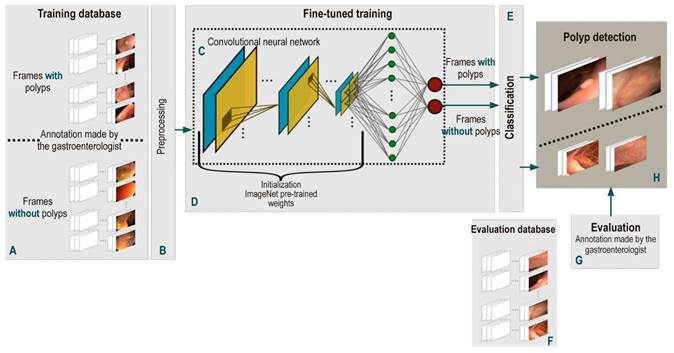
Figure 1 Flow diagram of the automatic polyp detection method proposed here. First, a frame-by-frame annotated database of colonoscopy videos (A) was created. All these frames are individually pre-processed (B) to feed the CNN-based models (C). This model is trained by fine-tuning some pre-trained weights with millions of natural images (D). Once the network is trained, its performance for detecting polyps (H) is evaluated with a test database (F) and the results obtained are compared with the annotations of an expert (G).
Acquisition and preprocessing protocol
Performing a frame-by-frame pre-processing of the video is required to reduce the effect of the numerous noise sources in acquisition process of different colonoscopes and the physiological conditions of the colon and the rectum. First, each frame is normalized using a mean of 0 and a standard deviation (SD) of 1, so that characteristics extracted are comparable between frames. Then, depending on the capture device, frames have different spatial resolutions, so each frame is scaled to 300 x 300 pixels, so that all have the same image grid.
CNN architecture
The main unit of these architectures is the neuron, which provides an output as a function of the inputs to it. An array of neurons creates a layer or block, and a network is composed of several elementary blocks arranged as follows: several pairs of convolutional (Figure 1C, blue box) and pooling (Figure 1C, yellow box) layers that deliver a vector of image features, followed by a set of fully-connected layers (Figure 1C, green circles) responsible for calculating the probability that a set of features has of belonging to a certain class, and ends with an activation layer (Figure 1C, red circles), in which the probabilities that were obtained are normalized and the desired binary classification is achieved. These blocks have the following functions:
Convolutional layers: they are responsible for Identifying local features throughout the image such as shape, border, and texture patterns, which are vital for the description of polyps. This layer connects a subset of neighboring pixels of the image or neurons to all nodes of the first convolutional layer. One of these layers or convolutional kernel is distinguished by the specific weights of each node; when operated on a specific region of the image, it provides a map of characteristics of said region.
Pooling layers: they reduce computational complexity, which in turn decreases the size of the features in convolutional layers and, this way, a hierarchical set of the characteristic maps of the image is obtained.
Fully-connected layers: This layer connects all the neurons in the previous layer to all the neurons in the next layer. The previous layer is a flat or vector representation of the maps of characteristics that were obtained. The number of neurons in the next layer is determined by the number of classes that need to be classified. Finally, the fully-connected layer provides a vote to determine whether an image belongs to a specific class or not.
Activation function: it normalizes the probabilities obtained from fully connected layers according to a specific function, where a probability of 0 to 1 is obtained.
A particular architecture consists of an array of modules containing different configurations and orders of fundamental blocks explained above, and the result obtained by each neuron is known as gradient. In this work, three highly evaluated and validated state-of-the-art architectures were used: InceptionV3, Vgg16 and ResNet50. Each of them is described below.
InceptionV3: it consists of 48 layers with 24 million parameters. These layers are largely grouped into 11 modules, in which features are extracted at multiple levels. Each module is composed of a given configuration of convolutional and pooling layers, rectified by the rectifier linear unit (ReLu) function. It ends with an activation function known as the normalized exponential function (softmax) function17.
Vgg16: it is organized in 16 layers for a total of 138 000 parameters. Of these 16 layers, 13 are convolutional layers, with a pooling layer (in some of them), and 2 are fully-connected layers; it ends with a normalized exponential activation function. This architecture is notable for using small 3 x 3 size filters in convolutional layers. Compared to most architectures, its computational cost is lower18.
ResNet50: it consists of 50 layers with 26 million parameters. This architecture is built based on the concept of residual networks. In very deep architectures such as ResNet50, the propagated gradient usually vanishes in the last layers. To avoid this, certain layers are trained with the residual of the gradient obtained in said layer and the gradient obtained in a layer placed two positions before. This architecture ends with a normalized exponential activation function19.
Fine-tuned training
High class classification performance depends largely on the number of annotated images and the way weights are initiated to train CNNs. A colonoscopy has approximately 12 000 frames per video, so the availability of annotated image databases is limited. This way, training with a limited number of data and initiating the network weights randomly, as it is generally done, results in a failed training process. To avoid this drawback, weights (transfer learning) from networks of the same type, which have been previously trained for another classification problem in natural images, are used with databases containing large numbers of annotated images. The reason why this is done in this way is that, even though natural and colonoscopy images are different, their statistical structure is similar, as well as the construction of primitives representing the objects. In these circumstances, the networks trained to recognize objects in natural images are used as an initial condition to train these networks to detect polyps.
These weights are used by means of a process called fine-tuning, in which the entire pre-trained network is taken and the last fully-connected layer is removed. This layer is replaced by a new one, which has the same number of neurons as the number of classes in the classification task (polyp-nonpolyp) and is initialized with the weights of the pre-trained network. Then, the last layer is trained first and, subsequently, the weights of the remaining layers of the network are updated in an iterative process; this methodology is known as backpropagation. Each iteration of this training is performed using a certain number of samples or batches of the training images. This process ends when the network has been trained with all the samples of the set, which is known as a training epoch. The number of epochs is determined by the complexity of the samples to be classified. Finally, training ends when the probability of a training image is high and matches the annotated label.
Polyp detection
The trained network model is applied to a set of evaluation videos in which a label is classified and assigned: (1) frames with presence of polyps and (0) frames without presence of polyps. However, there are frames with structures that resemble the appearance of a polyp, such as bubbles produced by intestinal fluids. The model has a classification error in these frames, as it considers there is a lesion in them. When these errors are temporally analyzed, the fact that they occur as outliers (from 3 to 10 frames) in a small time window (60 frames or 2 seconds) is remarkable. Therefore, the classification performed by the network is temporally filtered and if at least 50 % of 60 contiguous frames are classified as without presence of polyp, the remaining frames are filtered and given a new label: frames without presence of polyp. Finally, a polyp is detected when the proposed method classifies an image as a frame with presence of polyp or positive class.
Databases
The purpose of building the database in this paper was to capture the greatest variability of a colonoscopy procedure. With this in mind, sequences from different gastroenterology centers containing polypoid and non-polypoid lesions of varying sizes (morphology and location in the colon), and examinations performed by different experts and capture devices were collected to train and evaluate the proposed approach. These databases are described below.
ASU-Mayo Clinic Colonoscopy Video Database
This data set was built in the Department of Gastroenterology at the Mayo Clinic in Arizona, USA. It consists of 20 colonoscopy sequences divided into 10 with presence of polyps and 10 without polyps. Annotations were made by gastroenterology students and validated by an experienced specialist. This colonoscopy sequence collection has been frequently used in the relevant literature and it was used as database in the “2015 ISBI Grand Challenge on Automatic Polyp Detection in Colonoscopy Videos” event20.
CVC-ColonDB
It consists of 15 short sequences of different lesions amounting to a total of 300 frames. Lesions in this collection have high variability and their detection is highly difficult, as they are quite similar to healthy regions. Each frame contains notes made by an expert gastroenterologist. This database was built at the Hospital Clinic de Barcelona, Spain13.
CVC-ClinicDB
It is composed of 29 short sequences with different lesions for a total of 612 frames annotated by an expert. This database was used by the training set of the MICCAI 2015 Sub-Challenge on Automatic Polyp Detection Challenge in Colonoscopy Videos event. It was built at the Hospital Clinic de Barcelona, Spain21.
ETISLarib Polyp DB
It presents 196 images with polyps, and each image has annotations made by an expert. This database was used in the test set for the MICCAI 2015 Sub-Challenge on Automatic Polyp Detection Challenge in Colonoscopy Videos event22.
The Kvasir Dataset
This is a database that was created at Vestre Viken Health Trust (VV), Norway, using data collected through endoscopic equipment. Images are annotated by one or more medical experts from VV and the Cancer Registry of Norway (CRN). The data set consists of images with different resolutions ranging from 720 x 576 to 1920 x 1072 pixels20.
HU-DB
This database was built at the Hospital Universitario Nacional, in Bogotá and consists of 253 videos of colonoscopies with a total of 233 lesions. Each frame of the videos contains annotations made by an expert in performing colonoscopies with about 20 years of experience and more than 50 000 colonoscopies performed.
Each of these videos was captured at 30 frames per second and at a spatial resolution of 895 x 718, 574 x 480, and 583 x 457. A database with a total of 1875 cases and 48 573 frames with presence of polyps and 74 548 without polyps was created. Each frame in these videos was classified by an expert as positive if a polyp was present, or negative when there was no presence of a polyp. The number of videos and frames used in this work are summarized per database in Table 1.
Table 1 Description of the number of videos or cases and frames of colonoscopy videos used in this work by database*
*The consolidation of several databases to train and evaluate the methodology proposed here allows covering a large variability of lesions.
Ethical considerations
This study complies with the provisions of Resolution No. ° 008430 of 1993, which establishes scientific, technical and administrative standards for conducting research involving human beings (article 11). In accordance with said resolution, this is a minimal risk research, provided that only digital images, which are generated from anonymized colonoscopy videos, were required for its development, that is, there is no way to know the name or identification of the subjects included in the study.
Results
InceptionV3, Resnet50 and Vgg16 were the CNNs used in this work. Labels assigned by each of these networks were compared with the notes made by the specialists in each frame. The following experimental setup and evaluation methodology were applied to each architecture.
Experimental setup
CNNs were previously trained using images from the public ImageNET database, which contains approximately 14 million natural images. The resulting weights are used to initiate a new colonoscopy frame training process by means of the fine-tuning methodology. This method updates the weights, training the network with the colonoscopy database. The update of the weights was performed with 120 epochs over the entire training set. Each epoch trained the model by taking a batch of 32 frames until all frames were fully covered. The decision threshold was manually adjusted for each networks in order to maintain a balance in the classification performance for both classes. The following training scheme was established: 70% of the database for training purposes and 30% to make validations with respect to the number of cases, that is, data are separated from the very beginning and the training, validation and test data are never mixed. Networks were trained and validated with 213 cases (24 668 frames) with polyps and 36 videos (27 534 frames) without polyps in total. The evaluation process was carried out with 103 videos (23 831 pictures) with polyps and 25 videos (47 013 pictures) without polyps. A detailed account of this data set is shown in Table 2.
Table 2 Description of the number of sequences and frames selected from each database to evaluate the performance of the proposed methodology*
| Database | Number of videos | Frames | ||
|---|---|---|---|---|
| Polyp | No polyp | Polyp | No polyp | |
| ASU-May | 5 | 2 | 2124 | 2553 |
| CVC-ClinicDB | 9 | 0 | 191 | 0 |
| CVC-ColonDB | 4 | 0 | 145 | 0 |
| ETIS | 7 | 0 | 45 | 0 |
| Kvasir | 78 | 23 | 21 326 | 44 460 |
| HU | 103 | 25 | 23 831 | 47 013 |
*This corresponds to approximately 30% of the entire database.
Quantitative assessment
The approach proposed here automatically detects polyps in colonoscopy videos. This task is defined as a binary classification problem. This method assigns a label to each frame as negative class (a frame that does not contain a polyp) or positive class (a frame that contains a polyp). In order to evaluate the performance of this task, the estimated or predicted label is compared with the label annotated by the expert. This comparison allows for the calculation of the confusion matrix, which accounts for the following:
True positives (TP): the number of frames that were correctly classified as positive class by the model.
True negatives (TN): the number of frames that were correctly classified as negative class by the model.
False positives (FP): the number of frames that were incorrectly classified as positive class by the model.
False negatives (FN): the number of frames that were incorrectly classified as negative class by the model.
Using the confusion matrix, 4 classification metrics that evaluate the performance of the method for classifying frames with (positive class) and without (negative class) polyps independently, as well as the predictive power in both classes in general, were selected and calculated:
Sensitivity measures the proportion of frames containing polyps that were correctly classified.
Specificity calculates the proportion of frames that do not contain polyps that were correctly classified.
Precision indicates the predictive power of the method to classify frames with presence of polyps.
Accuracy is the rate of frames that were correctly classified based on the total number of frames.
The results obtained are presented according to each deep learning architecture described in the methodology section. Table 3 shows the results obtained for each architecture.
Table 3 Results obtained by the proposed method*
| Metric | InceptionV3 | Resnet50 | Vgg16 |
|---|---|---|---|
| Accuracy | 0,81 | 0,77 | 0,73 |
| Sensitivity | 0,82 | 0,89 | 0,81 |
| Specificity | 0,81 | 0,71 | 0,70 |
| F1 Score | 0,67 | 0,59 | 0,56 |
| Puntaje F1 | 0,74 | 0,71 | 0,66 |
| ROC (area under the curve) | 0,85 | 0,87 | 0,81 |
*Columns specify each architecture under evaluation, while rows specify each of the metrics that were used.
On the one hand, although most of these architectures show and outstanding performance in the classification task, Resnet50 architecture has the best metrics in terms of how well it detected positive class frames or frames with polyps, with a sensitivity of 0.89. On the other hand, InceptionV3 architecture had the best performance in terms of detecting negative class frames or frames without polyps, with a specificity of 0.81. Receiver operating characteristic (ROC) curves were built for each architecture to evaluate their performance in a more detailed way. This representation seeks to analyze how the models classify the images in terms of specificity and sensitivity by varying the decision threshold depending on the probabilities provided by the model. As can be seen in Figure 2, Resnet50 architecture has the best performance in separating the classes regardless of the decision threshold. This means that this architecture achieved a better generalization of both intra- and inter-class variability.
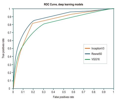
Figure 2 ROC curves for each of the evaluated architectures. The orange line corresponds to the InceptionV3 architecture curve; the blue line, to the Resnet50 architecture, and the green line, to the Vgg16 architecture. The Resnet50 architecture shows a better performance, with an area under the curve of 0.87.
Discussion
The detection of adenomatous polyps is the main quality indicator in a colonoscopy, since it is a fundamental marker for the detection and prevention of CRC. In many countries, the quality of a gastroenterologist is measured by the number of these polyps they detect in all the colonoscopies they have performed, which on average is around 25% for expert gastroenterologists, but it can be as low as 10% for inexperienced gastroenterologists, which results in more adenomas undetected when the latter perform a colonoscopy.
Several studies10-12 report that 26% of polyps are not detected during colonoscopies, which may contribute to the occurrence of more CRC cases. In this sense, by 2018, there were 1.8 million new cases of CRC worldwide according to the International Agency for Research on Cancer1. This loss rate is caused by several factors affecting an adequate examination of the colon, including the experience and level of concentration (associated with fatigue) of the expert during a whole working day, the physiological conditions of the colon such as blind spots in the haustra and the difficult placement of the colonoscope due to the colon motility, and the patient’s preparation for the procedure, which determines how observable the colon walls are23. Most of these factors allow concluding that colonoscopy is a procedure that highly depends on human factor, and therefore there is a need for second readers that are not affected by these factors. The use of computational tools for polyp detection in clinical practice would help confirm the findings made by the expert, and, more importantly, warn about the possible presence of lesions that were not detected by the expert. In this way, these tools would contribute to decreasing the rates of undetected polyps and, therefore, the incidence of CRC.
The challenge that supporting CRC diagnosis with computer vision tools entails has been addressed as follows:
detection, defined as the frame-by-frame binary classification of a video into positive class (with polyps) and negative class (without polyps);
localization, as the coarse delineation (by means of a box) of the lesion on an image containing a polyp;
segmentation, as a fine delineation of the lesion (outlining the edge of the polyp).
Polyp detection is the first and foremost task gastroenterologists must face. Post-detection tasks (localization and segmentation) are useful processes for the expert when the lesion has been already detected and its morphological description, based on medical guidelines such as the Paris Classification6, is required. This classification allows the gastroenterologist to make decisions regarding the surgical management of the disease in the short and long term. Consequently, these tasks depend entirely on how accurate the detection is; therefore, the methodology proposed here focuses on the main task required to be performed by the expert: obtaining colonoscopy frames with the presence of lesions. Furthermore, in the relevant literature, papers addressing these tasks13-15 have described limitations to present a single flow encompassing at least two of these task. These studies use different methodologies for each task, as each has its own level of complexity. In general, contextual or overall relationships are measured in the whole image to detect frames with polyps, while in the localization and segmentation tasks, local relationships at the pixel level are analyzed.
This paper presents a robust strategy for polyp detection, solved as a classification problem. Deep networks for classification tasks are methods that were formulated decades ago, but they had not been exploited until recently because computing power and availability of annotated databases were limited. In the last 5 years, the use of these models has increased dramatically thanks to technological advancement that now make possible a large amount of parallel processing and the publication of databases with millions of images such as ImageNet. This has made possible the design of highly complex networks and their exhaustive training, thus obtaining a high performance in classification tasks, since they allow modeling a high variability of shapes, colors and textures. However, in the medical field, there was no a large amount of annotated public data, so using these methods to solve disease detection or classification problems had not been considered.
The development of transfer learning techniques solved the shortage of medical data. The weights of networks trained with millions of natural images were used to initialize new networks and train them with a much smaller amount of different data, such as colonoscopy images. State-of-the-art studies that have used this method show that it has the ability to adequately generalize the high variability of frames with and without polypoid lesions in colonoscopy images extracted from a particular database. However, the different types of lesions and the physiological conditions typical of the large bowel are not the only source of variability. The less the expertise of the specialist, the more the probability of a higher number noisy frames in the video as a result of occlusions and abrupt movements made while handling the colonoscope. Additionally, capture devices vary in terms of light sources and camera viewing angles. Therefore, training and validating networks with databases obtained from a single gastroenterology service, as is the case of state-of-the-art works describing outstanding performances13-15, does not cover all the variability that colonoscopy image classification involves.
Bearing this in mind, a set of training videos with a high variability was consolidated in this work by gathering sequences from different databases; it should be noted that a data set like the one described here has not been presented in the state-of-the-art works. The set used to train this approach includes lesions of different sizes, shapes, and in different locations; colonoscopies performed by several gastroenterological experts, together with their notes, as well as videos recorded using different colonoscopy units. Despite such variability, the method proposed here showed a sensitivity of 0.89 and a specificity of 0.71 in the task of detecting polyps in colonoscopy sequences.
Conclusions
Deep learning methodologies are currently a promising option in the field of medical classification tasks. The advance of technology, along with the constant design and evaluation of networks, has allowed for the consolidation of a set of methods and flows enabling such networks to have a high performance. The results obtained in this work show that the networks evaluated here can be routinely used as second readers in colonoscopy services.
The fact that these networks adequately generalize the high variability of colonoscopy videos is remarkable. The results obtained here show that the proposed method can remarkably differentiate images with and without presence of polyps, regardless of the particular clinical protocol used for the recording of the video, that is, regardless of the expert performing the procedure and the capturing device. This method could be useful in decreasing the gap between expert and inexperienced gastroenterologists regarding adenoma detection rate.
Future works should address the implementation of the approach proposed here in full colonoscopies and evaluate if it is possible to use it in real time, as well as to develop a strategy that allows it not only detecting the lesion, but also delimiting it within the frame.

