


 English (pdf)
 Article in xml format
 Article references
 Send this article by e-mail
 Cited by SciELO
  Cited by Google
  Similars in
SciELO
Similars in
SciELO  Similars in Google
 Permalink
1. Introduction
Series wound DC motors are electrical machines in which the windings of armature and field are in series . As a consequence, when they are compared with any other DC motor, the series wound DC motor has the greater load torque per ampere of current supplied 1. The series connection of the windings generates two nonlinearities in its dynamics. On the one hand the voltage induced in its windings depends on the product between the current and the angular velocity, and on the other hand, the angular acceleration depends on the square of the current 2.
Velocity control for series wound DC motors has been the target of numerous researches that started in the decade of the 70's 3,4 and that have continue to the present days. Some recent works on the subject are: the nonlinear PI control proposed in 5, the fuzzy control based on the inference method of Takagi-Sugeno 6, the control without velocity sensor using an observer based on the algorithm of Super Twisting 7 and the control with artificial neural networks 8. In all of the above cases and in other less recent articles as 9,10,11,12,13, the proposed controllers are non-linear given the dynamics of the series wound DC motors .
Regarding the linear/nonlinear dichotomy there have been numerous comparative analyses applied to: wind tunnels 14, wind turbines 15,16 and fuel cells 17. However, to the best of our knowledge, for the case of series wound DC motors there has not been a comparison between linear and non-linear techniques. It is important to make this comparison to find out under what conditions a technique presents a superior performance over the other one and thus have the certainty when it is useful to implement non-linear controllers, which have greater complexity.
For this reason, in this article it is determined under what conditions the performance of a linear controller can be similar to the non-linear ones. In this aim, a comparison is made between the energy associated with the control effort and with the tracking error. The evaluation of the previous index was obtained when implementing a linear controller in the MS150 Feedback module and two non-linear controllers (feedback linearizing and sliding mode controls). The experimental results show that for velocities near to the operation point around the linear was obtained, the performance of the linear controller is superior than the one presented by the two non-linear ones.
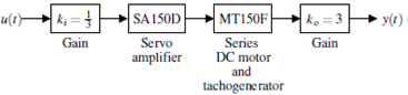
This article is organized as it follows: In section 2 it is described the MS150 module for Feedback on which was made the implementation of the controllers to be compared. Section 3 presents the dynamic model of the series wound DC motor. In section 4 it is estimated the parameters of the linearized model of the motor and the corresponding controller is designed. Section 5 deals with the estimation of the parameters of the nonlinear model as well as the design of two controllers, one using feedback linearizing control and the other one by means of first order sliding mode control. Section 6 compares the results obtained from the implementation of the linear controller and the two non-linear ones through the use of two performance indexes. The first one based on the velocity tracking error and the second one on control effort. Finally, section 7 presents the conclusions of the work.
2. Nonlinear model of the DC series motor
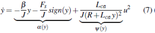
Consider the series wound DC motor depicted in Figure 1. In such a figure Rf represents the field resistance, Ra the armature resistance, Lf the inductance of the field, Lf the inductance of armature, J the moment of inertia associated to the charge, u(t) the voltage applied to the armature circuit, i(t) the current flowing through the windings, w (t) the angular velocity, f (w) the friction torque composed by the viscous and dry components respectively given by β w and Fs sign(w ), ε (t) = KLfi(t ) w(t) the induced voltage.
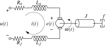
Based on the Kirchhoff's voltage law, Newton's law for rotational systems and the principle of energy conservation, it is obtained the following state space model 18
Where R = Rf + Ra , L = Lf + La and Lca = KLf . The equation (1) will be the starting point for the design of the linear controller and the non-linear ones.
3. Linear identification and control
3.1. Linear identification
For the acquisition of input-output data required for the identification of the parameters of the motor, the setting presented in Figure 2 was used. Figure 3 shows the input and output signals obtained. The sampling time used was 30 ms, the number of samples taken was 1000 and the base value of the excitation was 3.25 volts which corresponds to the 65 % of the maximum operating velocity.
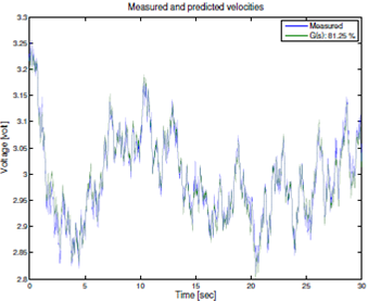
From the linearization of (1), it was concluded that the linear model that represents the motor would be a transfer function of second order without leading zeros. The model estimated from the data in Figure 3 was:
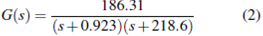
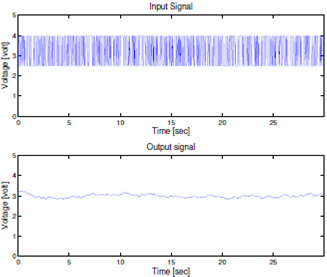
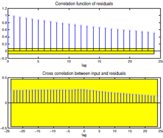
Figure 4 shows that the adjustment level between the measured velocity and the predicted by the transfer function in (2) was the 81.25 %. In Figure 5 are presented the results of the statistical validation of (2). In the upper part of Figure 5 it is shown that although the residual do not constitute a pure white noise signal because (2) does not involve a noise model, the lower part of the figure shows evidence that the correlation between residuals and the input signal is not statistically significant, indicating that the obtained G(s) is valid.
3.2. Linear control
Since (2) contains a pole approximately 218 times faster than the other, a first-order model is used for the controller design. The reduced model is given by the following equation
The expression (4) is used for the controller design.
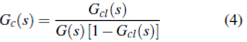
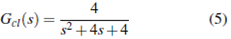
In (4), Gcl(s) is the transfer function that describes the desired behavior of the closed loop system, G(s) is the model of the process used to design the controller and Gc(s) is the obtained controller. The Gcl(s) described by (5) allows to obtain a settling time of 2 seconds and a damping factor of 1.
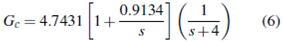
When introducing the G( s) and the Gcl(s) respectively given by (3) and (5) in (4) the following controller is obtained:
4. Nonlinear identification and control
4.1. Nonlinear identification
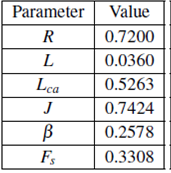
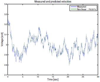
The parameters R, L, Lca, J, β and Fs of the model (1) were estimated, as in the linear case, using the data presented in Figure 3 and performing a least squares adjustment. Figure 6 shows that the level of adjustment between the measured velocity and the predicted by (1) was of 79.59 %. The numerical values of the parameters obtained are listed in table 1.
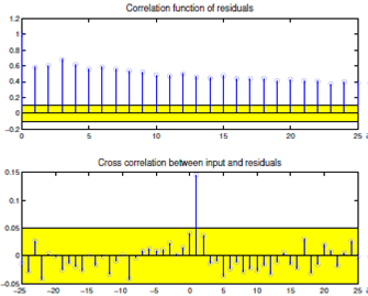
As in the linear case, there was also a statistical validation of the model. Figure 7 presents the residual analysis (upper figure) and a correlation residue-excitation analysis (bottom figure). Of these figures, it can be concluded that although the residuals do not constitute a white noise signal and despite finding a strong correlation between ep(k) y u(k - 1), the percentage of adjustment between the measured data and the data predicted by the model obtained is relatively high.
4.2. Feedback Linearized Control
Once the parameters of the nonlinear model were identified, the design of the controller using an output feedback linearization technique was made. To design this controller, the dynamic of the electrical component was not taken into account since it is much faster than the mechanical component. Evidence of this is that the G(s) transfer function has a pole approximately 218 times faster than the other. Additionally, if this dynamic was to be taken into account it would require an observer that considers the input current to the motor which would increase the complexity of the design. When assuming  = 0 in the model (1) and pointing out that the measured variable is the velocity (y = w), the following model is obtained
To cancel the nonlinearities present in (7) the following control law is selected,
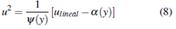
When replacing(8) in (7) the simple integrator linear model  = ulineal
is obtained, to which it is possible to apply any linear control technique. For this implementation, the proportional-integral action described in (9) was selected.
= ulineal
is obtained, to which it is possible to apply any linear control technique. For this implementation, the proportional-integral action described in (9) was selected.
Where e(t) is the velocity tracking error,
Bp
is the proportional band and
Ti
is the integral time. The values of these two constants are
Bp =
20, and
Ti =
 .
.
4.3. First order sliding mode control
The design of the sliding mode controller is mainly based on the selection of a switching surface suitable for the discontinuous control (19). Taking into account the first-order reduced model of the equation (7), which shows that it is necessary to derive the output y(t) only once to obtain u(t), the control law defined in equation (10) is chosen.

Being sign the function of the switching surface of the control law, ed (t) an approximation of the derivative of the error signal and X a coefficient that determines the weight of the error derivative on the control law. X in 0.1 is chosen.
5. Results and discussion
In order to carry out the comparative study, necessary as a main purpose of the present article, the controllers described in (6), (8) and (10) were discretized. With the resulting difference equations an implementation in C language was made on an Arduino MEGA 2560 board. In all three cases the velocity setpoint was a staircase type signal that varied from 0 % to 100 % with an increment of 10 % every 500 samples as shown in table 2.
Table 2 Stair signal used as a setpoint for the closed loop system. Setpoint is increased by 10% after 500 samples (1.5 seconds).
| Sample | Setpoint |
| 1-500 | 0% |
| 501-1000 | 10% |
| 1001-1500 | 20% |
| 1501-2000 | 30% |
| 2001-2500 | 40% |
| 2501-3000 | 50% |
| 3001-3500 | 60% |
| 3501-4000 | 70% |
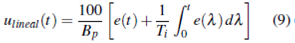
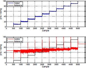
5.1. Obtained results for the linear controller
In the top of Figure 9, it can be observed that the output of the linear controller presents strong oscillations when the setpoint velocity is below 60%. However, once this value is exceeded, the overshoot and the output signal oscillation decrease considerably. In the bottom of Figure 9, it can be seen that the control effort reduces its oscillation when the reference velocity is increased above 80%.
5.2. Obtained results for the output feedback linearization control
Figure 11 shows that the controller output by output feedback has little oscillation at all points of operation. However, at low points of operation it presents a considerable overshoot and as operation velocity increases, the overshoot decreases visibly. Furthermore, it is observed that the oscillations of the control effort decrease while the operating velocity increases.
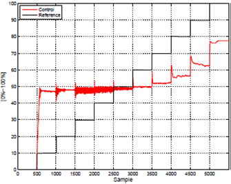
5.3. Obtained results for the sliding mode control
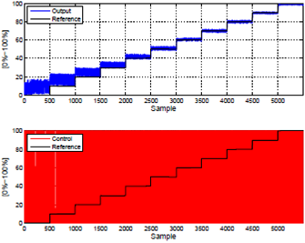
Figure 12 shows that the nonlinear controller has an oscillatory response in all operation points, this is attributed to the chosen sliding surface, which only takes one of two values (0% or 100%), impacting directly on the sharp oscillation of the control law.
5.4. Performance index
In order to make the comparison between the implemented controllers, two performance criteria respectively based on the tracking error and the control effort were defined.
Average of the sum of the square of the error:
Where N is the number of samples taken, r(k) is the reference signal and y(k) is the output signal.
Average of the sum of the square of the effort control:
Where u(k) is the control signal sent to the motor armature.
These criteria were applied by considering three scenarios based on the range in which the velocity set-point was varied. In the first scenario the setpoint remained on 60 % which was the value used to obtain the linear model of the system. In the second scenario the velocity setpoint ranged from 40 % to 80 % with an increment of 10 % every 500 samples. The third scenario was equal to the second one, but the variation on the setpoint was progressively carried out from 20% to 100%.
Table 3 shows the values obtained for the performance index (11) on each of the three considered scenarios. For the first scenario it is observed that the controller that has the lower mean square error is the linear and for scenarios 2 and 3 is the linearizing controller. Additionally it can be observed that for each of the three controllers considered the mean square error of the scenario 1 is lower than the one of the scenario 2, and this in turn, is less than the one reported for the scenario 3. This means that the index (11) grows by increasing the range of values in which the setpoint velocity is varied.
Table 3 Comparison between the mean square tracking error of each controller for the three considered scenarios. Scenario 1: r(k) = 0.6, Scenario 2: 0.4 < r(k) < 0.8, Scenario 3: 0.2 < r(k) < 1.0.
| Controller | Scenario 1 | Scenario 2 | Scenario 3 |
| Linear | 3.8587e-01 | 2.1608e+00 | 2.7129e+00 |
| Feedback | 5.7097e-01 | 6.5195e-01 | 7.0960e-01 |
| Sliding | 1.8385e+00 | 2.8995e+00 | 8.2093e+00 |
Table 4 shows the ratio between the performance index (11) of the non-linear controllers and linear one. It can be seen how as the velocity setpoints take distance from the point around which the linear model was obtained, the monitoring mean square error of the linearizing controller decreases with respect to the linear control.
Table 4 Mean square tracking error of the nonlinear controllers with respect to the linear controller for the three scenarios. Scenario 1: r(k) = 0.6, Scenario 2: 0.4 < r(k) < 0.8, Scenario 3: 0.2 < r(k) < 1.0.
| Controller | Scenario 1 | Scenario 2 | Scenario 3 |
| Feedback | 1.4797 | 0.3017 | 0.2616 |
| Sliding | 4.7646 | 1.3419 | 3.0260 |
Table 5 presents the values obtained for the performance index associated to the control effort (12). For the first scenario it is observed that the controller that has the lowest mean square value is the linear one, and for scenarios 2 and 3 it is the linearizing controller. Table 6 shows the ratio between the performance index (12) of the non-linear controllers and the linear one. In the same way that for the monitoring error, the index (12) of the linearizing controller decreases as the velocity setpoints take distance from the point around which the linear model was obtained.
Table 5 Comparison between the mean square control effort of each controller for the three scenarios. Scenario 1: r(k) = 0.6, Scenario 2: 0.4  r(k)
r(k) 0.8, Scenario 3: 0.2 r(k)1.0.
| Controller | Scenario 1 | Scenario 2 | Scenario 3 |
| Linear | 2.4847e+03 | 2.6167e+03 | 3.0613e+03 |
| Feedback | 2.6075e+03 | 2.6020e+03 | 2.8747e+03 |
| Sliding | 3.3400e+03 | 3.5760e+03 | 3.9333e+03 |
Table 6 Mean square control effort of the nonlinear controllers with respect to the linear controller for the three scenarios. Scenario 1: r(k) = 0.6, Scenario 2: 0.4 ≤ r(k) ≤ 0.8, Scenario 3: 0.2 ≤ r(k) ≤ 1.0.
| Controller | Scenario 1 | Scenario 2 | Scenario 3 |
| Feedback | 1.0494 | 0.9944 | 0.9390 |
| Sliding | 1.3442 | 1.3666 | 1.2849 |
6. Conclusion
For Series wound DC motors it was observed that when conducting experiments with reference values far away and relatively close to the operation point on which the model was identified, the linearizing controller presents a significant advantage over other controllers. However, despite the complexity of its control law, it has an inferior performance with respect to its linear counterpart, when experiments are carried out at operation velocities very close to the operation point.

