


 English (pdf)
 Article in xml format
 Article references
 Send this article by e-mail
 Cited by SciELO
  Cited by Google
  Similars in
SciELO
Similars in
SciELO  Similars in Google
 Permalink
Introduction
Job sequencing is one of the main challenges faced by the people in charge of planning and scheduling production.. This is due mostly to the combinatory nature of the task and the fact that these types of problems can be classified as NP-Hard ones 1, which requires the development of advanced algorithms that may offer nearly optimal solutions, thus allowing for an efficient use of computational resources.
On another note, static models (such as bifurcation and dimensioning) have approached job scheduling without contemplating the appearance of unexpected events in the execution of production processes. This has created a gap between theoretical models and real manufacturing environments 2.
Hence, this work studies the Job Shop Scheduling Problem (JSSP) from a rescheduling-oriented perspective, seeking a better representation of the actual conditions of manufacturing environments. Rescheduling is a process that can react to unexpected events as a part of the dynamics of said environments 3. In this sense, the Job Shop Rescheduling Problem (JSRP) 4)-(7 is conceived as a problem of higher complexity.Studies focused on the rescheduling of manufacturing systems are wide and diverse. Therefore, this work is framed within the search for methods to fix production timetables that have been affected by an unexpected event 3. The method developed in the subsequent sections is based on the architecture of a transgenic algorithm 8, which is characterized by metaheuristics applied to diverse problems of high complexity, leading to competitive results compared to more renowned techniques 9)-(14).
The main objective was to develop a computational algorithm based on the metaphor of transgenic computation 53 which allows production schedulers to generate high-quality timetables in terms of efficiency and stability while also being able to react to unexpected events or interruptions arising during the execution of said timetables, thus mitigating the impact on the performance of the manufacturing system.
Proposal
2.1. Job Shop Scheduling Problem
Sequencing problems can be as diverse as manufacturing environments. The JSSP is one of the most studied topics in the research field of operations and computer science. This is mostly due to its relationship with production planning activities within the industry. The JSSP is recognized as an NP-Hard problem 1 and is considered to be among the highly complex and unmanageable optimization problems 15),(55.
JSSP is defined as a manufacturing environment containing a set J = {1, . . . , j, . . . , n} of n jobs that must be scheduled in a set M = {1, . . . , i, . . . , m} of m machines. Each job has a technological sequence of machines (stages) for it to be processed. The use of machine i for the processing of job j is denoted as operation O ij with a duration equal to t ij , which is known as the processing time. Furthermore, the problem revolves around constraints and suppositions such as the following:
Each machine can only process one job at a time.
Each job can only be processed by one machine at a time.
Jobs must only be processed once in each machine.
The technological sequence of each job has been completely defined.
The machines are always available and never interrupted.
The problem consists of determining the sequence of operations to be defined for the machines in order to minimize the makespan (C max ), whose value is the time necessary to complete all the operations. The JSSP with makespan as the target can be mathematically described via Eqs. (1), (2), (3), (4), and (5):


where r ij is the time at which operation O ij starts, N is the set of all operations O ij , and A is the set of all constraints given by the technological sequence of each job, such as O ij → O kj , which requires job j to be processed by machine i before being processed by machine k. This formulation of the JSSP is called disjoint scheduling given the third set of constraints 16. Furthermore, the JSSP can be defined as an integer scheduling problem 17.
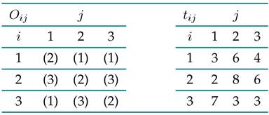
An instance of three jobs for three machines (3 × 3) of JSSP is represented as: As evidenced in this table, matrix O ij describes the order in which the jobs for each machine are processed. For instance, job 1 (j = 1) has the following technological sequence: (1) O 31 → (2) O 11 → (3) O 21. Matrix t ij contains the processing times of each operation O ij .
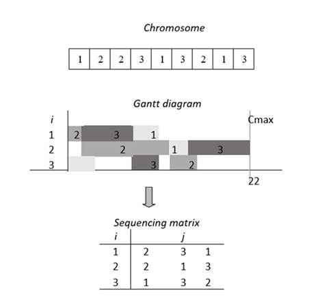
There are different representations of the solution for this problem. The Gantt diagram is one of the most commonly used forms in this regard. Fig. 1 shows an example of the representation obtained for a solution of the instance in Table I.
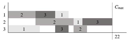
The Gantt diagram depicts what is known as the production timetable. It shows a feasible solution to the JSSP when all constraints are satisfied. It is worth noting that this definition of the JSSP corresponds to a theoretical problem that constitutes one approximation to a more complex scenario.
On another note, researchers studying the JSSP have opted to define a set of assumptions and constraints, leading to a gap between theoretical models and real manufacturing environments (2).
Job Shop Rescheduling Problem
The definition of the JSSP described in the previous section is a deterministic and static sequencing model, as its parameters and variables are known beforehand and do not change over time. Thus, this model only represents an approximation of a real manufacturing environment, since the industry experiences some scenarios encompassing variables that are dynamic or have a high degree of uncertainty.
In this sense, when a production timetable is built, both the supervisors and the operators attempt to execute it as closely as possible. The issue lies in unexpected events that alter the execution of the current production timetable, causing it to become inappropriate and unmanageable. Said events are called interruptions and need to be treated swiftly in order to minimize any effects that can deteriorate the system performance 55. This is where rescheduling becomes the proper tool to handle interruptions and complete all scheduled jobs.
Rescheduling is defined as the process of updating the existing production timetable in response to the interruptions or changes 3, whose integration with the Job Shop manufacturing environment results in what is referenced in the literature as the Job Shop Rescheduling Problem (JSRP) (4)-(7.
Studies on rescheduling from different perspectives are numerous. The most common approaches are the following: (i) methods to fix a timetable that has been interrupted, (ii) methods to create robust timetables to face interruptions, and (iii) studies on how rescheduling policies affect the performance of dynamic manufacturing systems.
Some of the articles include, for instance, the study of the Job Shop environment under the dynamic arrival of new jobs, variations in processing times, and machine failure 18. Other authors, such as 19, propose an algorithm capable of predicting and absorbing the effects of interruptions while maintaining system performance. In 20, a genetic algorithm is applied to scheduling and rescheduling in a non-deterministic Job Shop environment.
Given that the studies on rescheduling are as numerous as they are diverse, this work adopts the rescheduling framework defined in 3. This framework allows for the understanding of rescheduling studies, in addition to classifying the technique discussed herein.
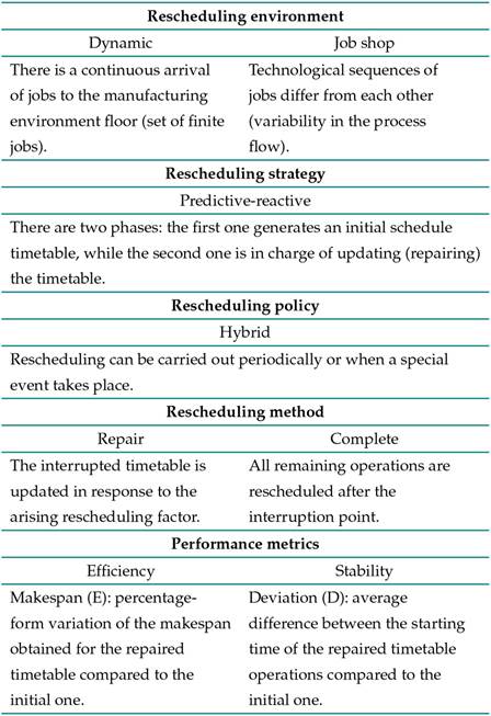
In order to properly narrow down the study of rescheduling in manufacturing environments, it is necessary to include an appropriate framework, given that its study can become widely diverse and complex depending on the scope defined by the researcher. According to 3, the rescheduling framework is composed of these elements: rescheduling environments, strategies, policies, and methods.
Rescheduling framework
Rescheduling environment refers to the set of jobs that must be scheduled. The environment can be static (finite set of jobs) or dynamic (infinite set of jobs). The environment can be deterministic (all the information is given) or stochastic (some information is uncertain). Dynamic environments may also be classified according to the variability in which the arrival takes place: without variability (cyclical production), with variability (flow shop), and with variability in the process flow (job shop).
Rescheduling strategies refer to how production is controlled in the aforementioned environments, whether timetables are generated or not. Two common strategies have been identified in this regard: dynamic sequencing and predictive-active sequencing. The former does not generate production timetables, since the jobs are dispatched when necessary, using the information available at the moment of dispatch and with the help of dispatch rules or theoretical control models for manufacturing systems. The second strategy is characterized by two phases: a predictive phase, during which the initial production timetable is generated; and a reactive phase, in which the production timetable is updated as a response to interruptions in order to minimize their impact on system performance. The predictive-reactive strategy includes three policies: periodic, given event, and hybrid. These refer to the moment of rescheduling.
Rescheduling methods describe how to generate and update production timetables 54. Two approaches have been proposed: the generation and repair of timetables. The generation of production timetables can be coordinated through different techniques, in the form of analytical, heuristic, or more complex algorithms. The timetable repair approach (i.e., update process) includes three main variants: right-shift rescheduling, partial rescheduling, and complete rescheduling.
In addition to the previously discussed elements, performance metrics are an important guideline in rescheduling studies. They can be classified into three groups: efficiency metrics, stability metrics, and timetable costs. The first group is made up of the most common time-based metrics, such as makespan, average delay, and average flow time. The second group refers to the variables that measure changes within a timetable in terms of launch times or the differences between sequences. Lastly, the cost variables include benefit according to the job, minimization of the total cost, and reduction of the work in process (WIP), among others.
Various techniques have been proposed in literature to solve the rescheduling problem in terms of the aforementioned performance metrics. Methods such as right-shift rescheduling 21, match-up 22, and Affected Operation Rescheduling (AOR) 23 are some of the most well-known group of heuristics and are characterized by a simple implementation process, which is however limited by the range of interruptions that they can face. Furthermore, these heuristics operate under the partial rescheduling strategy, which implies that they try to adhere to the preestablished timetable as much as possible after the interruption 24), (25.
On another note, complete rescheduling techniques seek to reschedule all remaining operations after the point of interruption 26), (27. Under the umbrella of this approach, diverse and sophisticated algorithms have been implemented, as is the case of genetic algorithms 4), (20),(53), (55, which are known to improve the efficiency of timetables while ignoring stability-related metrics.
In this sense, new techniques are constantly being developed to solve combinatorial problems. JSSP is no exception, since it belongs to this class even from the rescheduling (JSRP) viewpoint, implying that timetables require more quality over time with a rational use of computational resources. Hence, the next section exposes an algorithm that has offered many advantages in other problems of the same nature.
Transgenic algorithm
In the context of evolutionary computation, defined as the study of the foundations and applications of certain heuristic techniques based on natural evolution principles 28, a variety of algorithms have been developed to face highly complex problems such as the one discussed in the present work.
Since the appearance of genetic algorithms in the article titled Adaptation in natural and artificial systems29, techniques based on this metaphor have not been scarce. Some of them have inherited the basic structure of genetic algorithms to be combined with other local search techniques, paving the way for genetic/evolutionary hybrid algorithms 16), (30, Lamarckian genetic algorithms 31, or general memetic algorithms 32), (33.
The term memetic algorithm stems from the English term meme, coined by R. Dawkins as an analogy to the gene in the context of cultural evolution. 34 defines memes as the units of information coded and transmitted by non-genetic media. These definitions are relevant for the approach described in the subsequent section, which is based on the transgenic algorithm.
Transgenic computation (TC) is a metaphor derived from the use of memetic information (memes) and extra- and intracellular flows to plan and execute genetic manipulations in the context of evolutionary algorithms 8.
To the scope of evolutionary computation, TC brings the use of exogenous and endogenous information to infer the formation and modification processes of the individuals in a given population, to use intracellular flow as an operational mechanism in order to carry out the required manipulations amongst individuals, to explore new populational improvements using transgenic agents and competition between agents and individuals, and to guide the evolutionary process, allowing for the occurrence of evolutionary jumps 9. Further information on the basics of TC can be found in 8), (10),(11.
This method has been branched into two types of algorithms: the extra-intracellular transgenic algorithm (EITA) 12 and the proto-gen (ProtoG) algorithm 9. The most noticeable difference between them lies in the fact that the ProtoG algorithm does not have reproduction operators (mutation or cross), so it is not based on an extracellular approach 9.
The proposed algorithm is based on the ProtoG algorithm, whose structure and composition are detailed below.
As discussed with TC, transgenic algorithms are metaheuristics that insert information in a planned manner for improving genetic information. Their pillar lies in the intracellular paradigm, through agents that manipulate the genetic context. The information inserted by said agents is created and controlled via the epigenetic paradigm. These paradigms define the ProtoG algorithm per se, thus excluding the extracellular paradigm that uses sexual reproduction as the basis of information exchange between individuals 10.
In this algorithm, the chromosomes are exposed to a direct attack from the agents in the intracellular flow, which must compete against each other and the defense mechanisms of chromosomes in order to consolidate the transcription of their codes 11. In the computational context, said chromosomes are part of the population C of size q, where C = {1, . . . , c, . . . , q} is a function f called the fitness function. Each chromosome c is a chain of integer length h that represents a solution to the problem, such as f: c → R+, c = 1, . . . , q, where f returns a real value.
Chromosomic alterations are only carried out by transgenic agents, which makes them essential to the evolutionary process as the only source of intensification and diversification in the search process 9.
Transgenic agents are entities used by the algorithm to insert information into the genetic context. These agents manipulate chromosomes similarly to intracellular vectors used in genetic engineering. As an analogy to the terms used by microbiologists, there are four types of transgenic agents: plasmid, virus, recombined plasmid, and transposon 11.
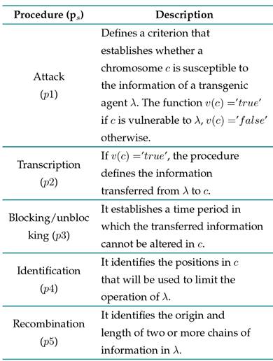
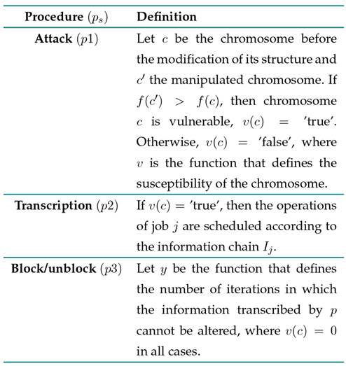
In the computational context, a transgenic agent λ is defined as a couple λ = (I, Φ), where I is a chain of information (corresponding to the memes) and Φ describes the manipulation method used by the agent. Φ = (p 1 , . . . , p s , . . . , p x ) where p s , s = 1, . . . , x, are the procedures that determine the behavior of the agents. Table II depicts the procedures of the manipulation method (extracted and adapted from 11).
In this sense, when the chain of information I of λ is a genetic code and its manipulation method uses procedures p 1 , p 2, and p 3 , λ is called a virus 11. In the case of the ProtoG algorithm, the mobile genetic particle (MGP) is a special case of virus where the virus lifetime (or blocking period) established by procedure p 3 is equal to zero, and the attack procedure p 1 only takes place when chromosome fitness is improved 9.
The difficulty of considering epigenetics in the context of evolutionary computation is discussed by 34. The initial work on this matter simply linked the memes to information obtained outside the extracellular flow 10. In memetic algorithms, according to 35 and 36, the epigenetics stage is mainly expressed through the improvement of chromosomes using local search procedures. This is where TC adopts a new approach, defining memes as memories with information that is stored, coded, and transmitted using non-genetic means, as stated by 33. Hence, memes can be used to adjust a chromosome or block of genes, or said memes could be subjected to competition and selection processes relevant to the cultural media 10.
Memes are units of information that can be spread by a culture in the same way that genes are disseminated through a genetic reservoir 37. The relationship between genes and memes is based on the fact that genes prescribe the epigenetic rules, which are regularities of sensorial perception and mental development that encourage and channel the acquisition of culture. Culture contributes to determining which prescribed genes survive and multiply from one generation to the next one. New properly sequenced genes alter the epigenetic rules of the population. The altered epigenetic rules change the direction and effectiveness of cultural acquisition channels by offering feedback to the coevolution ‘gene vs. meme’ process 38.
In the computational context, these epigenetic rules are simulated by a transgenic rule-based structure. The evolution control of a population of chromosomes, transgenic agents, and the information of a memetic base is composed of three classes of rules 10), (11.
Type 1 rules lead to the construction of information chain I, which is transported by the transgenic agents 11. These types of rules can have knowledge on any aspect of the problem, as well as previous knowledge stored in the memetic base (MB), which constitutes the storage bank of memes. Memes can be comprised of construction blocks or manipulation procedures 11. Type 2 rules define the information contained in I is transcribed into a chromosome, i.e., the operator used by λ. These types of rules can evolve in terms of the resistance shown by chromosomes. Type 3 rules are present throughout the process, defining which agents are used, the number of chromosomes under attack during a given iteration, the number of agents created, and the stopping criterion, among others 11, 12.
The ProtoG algorithm can be decomposed into two phases. The first one generates the construction blocks (memes) and codes them using transgenic agents. In the second phase, the agents compete to transcribe their information into the chromosomes and thus improve the solutions 9.
The implementation of the ProtoG algorithm improves the fitness of the chromosome population through the manipulation carried out by the transgenic agents. However, not only chromosomes evolve; memes also do. This process makes TC an informed and co-evolutionary search technique 9.
Transgenic algorithms, including ProtoG, have proven to be successful when compared to known techniques in the solution of high-complexity problems. Some of the problems tackled by this technique include the quadratic allocation problem (QAP) 9), (11, the traveling purchaser problem (TPP) 12, the graph coloring problem 12, and sequencing in flow-shop with permutation 13, among others 39), (40.
The pseudocode of the algorithm is the following (taken and adapted from 9,11):

Proposed algorithm
As discussed in Section 3, the proper definition of the scope of rescheduling requires an appropriate framework. The approach of this work lies in the methods used to repair a timetable that has been interrupted. Hence, it is important to initially define these interruptions, also known as rescheduling factors41), (42, which arise at a given time of the initial timetable known as the interruption point. This study contemplates all the rescheduling factors identified in the work of 43, as shown in Table III.
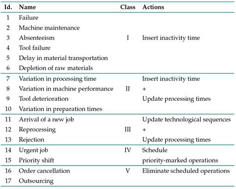
Given that rescheduling factors are a significantly wide group, they are classified into five classes. This classification is based on the general actions that would be needed to repair the interrupted timetable and meet the constraints imposed by the arising rescheduling factor. A description of the considered factors can be seen in 44.
Manufacturing environment
The rescheduling framework defined by 3 encompasses the elements of the proposed algorithm framework shown in Table IV.
Transgenic algorithm
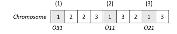
As stated in the field of evolutionary computing, one of the most important factors in the success of algorithms is the representation of the problem. In this sense, 16 conducted a study of the representation forms used in the application of genetic algorithms to solve the JSSP. In this case, operation-based representation was selected, which defines n jobs and m machines to create a chain (chromosome) of n × m positions (genes), where all operations of job j are distinguished by the same symbol (number) that appears exactly m times throughout the chain. Each appearance of the symbol that represents job j corresponds to an operation in the order of the technological sequence of said job. This representation method offers the advantage that all permutations in its elements provide a feasible solution to the JSSP, thus avoiding complex repair processes, as seen in other alternatives. An example of this representation is shown, using the instance data presented in the second section:
As seen in Fig. 2, each appearance of the number 1 (j = 1) refers to an operation in the technological sequence. This can be replicated for the remaining jobs. The representation can be useful during the elaboration of the Gantt diagram. The chromosome is read from left to right, where each position (gene) delivers the information of an operation O kj . The operation is inserted into the diagram by setting the starting time r kj as early as possible, i.e., by checking the conclusion time of the preceding operation O ij and not overlapping times with a previously inserted operation. Lastly, operation O kj is defined from r kj to r kj + t kj . An example of the aforementioned procedure can be seen in16.
After the representation of the solution is defined, the next task involves the design of the rescheduling method based on the ProtoG algorithm architecture for the previously defined manufacturing environment, which is divided into the following two stages:
The transgenic agents of the evolutionary process are defined in this stage. It is worth mentioning that these agents have been designed in terms of the JSSP features defined in the second section. The MGP is the agent chosen to carry out the genetic modifications. The composition and general structure of the designed agents is shown below.
Let λ = (I j , Φ) be a transgenic agent composed of an information chain I j = (g 1j , . . . , g ij , . . . , g mj ) or meme with length m, where the element g ij can represent one of the following elements: a position in the processing order, a preceding job, or an adjacent job, as suggested by the evolutionary process, which is taken as a reference to schedule job j in machine i, with i = 1, . . . , m and j J . Let Φ = (p 1 , p 2 , p 3), be the manipulation method of the agent composed of the procedures p with s = {1, 2, 3}. Table Vdefines each procedure.
Three agents were designed for this algorithm. They all inherit the previously defined composition and structure, and the only difference between them is the type of information (meme) that they carry. The following section describes how the epigenetic paradigm creates, stores, and controls this information in the MB to guide the evolutionary process.
As previously stated, there are three types of rules that represent this paradigm in the computational context. Recall that type 1 rules lead the construction of the information chain (meme) that is transported by the transgenic agent. This information is stored in the MB. To illustrate this process, Fig. 3 presents a diagram representing the flow of individuals from the population to the transformation of their information into memes. The process starts with the population of chromosomes. This population enters a selection process, where chromosomes with the best fitness are considered to continue with the process (This procedure is controlled by a factor that will be defined later).
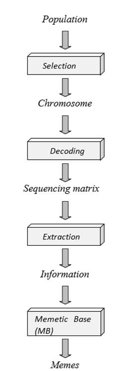
Once the chromosome has been selected, it undergoes a new procedure called decoding. This refers to the conversion of a chromosome into a convenient representation form, which is used to extract the information needed by the MB to create memes. The result of this decoding stage is the sequencing matrix, defined as an array of m rows by n columns, which represents the sequence in which the jobs will be processed by each machine. An example of said procedure is depicted in Fig. 4. The sequencing matrix is derived from the examination of the Gantt diagram linked to the chromosome. In the form of a matrix, this array summarizes the information related to the order in which the jobs of each machine will be processed.
Now that the decoding process has been detailed, the sequencing matrix becomes the main asset for the extraction procedure. It consists of obtaining key information from the structure of the given chromosome.
Once the information has been extracted, it is stored in the MB. The matrices that integrate said base are described below.
Let MB be a set of matrices MB = {Mp, Mr, Ma, Mb} that store specific information from the population of chromosomes C through an evolutionary process.
Mp is defined as the position matrix, where the element Mp ijl is the average makespan of the chromosomes that have scheduled the job j in the sequence of operations of machine i in position r, with i = 1, . . . , m, j = 1, . . . , n, r = 1, . . . , n.
Mr is defined as the precedence matrix, where element M rijl is the average makespan of the chromosomes that have scheduled the job j in machine i before job l with i = 1, . . . , m, j = 1, . . . , n, l = 1, . . . , n.
Ma is defined as the adjacency matrix, where the element M aijl is the average makespan of the chromosomes that have scheduled the job j in machine i exactly one position before the job l, with i = 1, . . . , m, j = 1, . . . , n, l = 1, . . . , n.
Memes are built based on the minimum values of matrices Mp, Mr, and Ma. The obtained memes are denoted as I pj (meme1), I rj (meme2), and I aj (meme3), respectively, where j ∈ J is a reference job chosen at random for the construction of the chain.
The last matrix that comprises the memetic base is Mb, defined as the meme matrix, where the previously defined memes are stored. Each meme is linked to an accumulative score S cw that is updated every time that the corresponding agent uses the meme to modify the structure of a chromosome. Said score is given by the function S cw (current) = S cw (previous) + (f (c ′ ) − f (c)), with w = {1, 2, 3}. Furthermore, memes have a counter defined by C ow , which adds one unit to its previous value each time that v(c) =’false’, i.e., when the chromosome is not vulnerable to the meme.
After defining the construction process of information chains Ij, type 2 rules are presented, which allow defining how the information contained in said chains is transcribed into the chromosomes. The transcription procedures of type p2 used by the designed agents are slightly different due to the type of information that they carry. The manipulation procedure consists of a positional exchange of genes within the chromosome, which are linked to the meme contained by the agent.
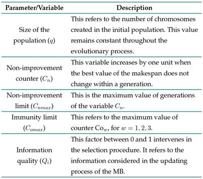
Lastly, type 3 rules are present throughout the evolutionary process, defining the parameters and criteria that dominate the operativity of the algorithm. Table VI summarizes the parameters and variables that complement the previously discussed terms. These are also necessary during the construction of the algorithm.
Consequently, the following criteria and rules are defined:
The creation of the initial population of chromosomes C is performed randomly, where each chromosome represents a solution to the JSSP.
Chromosomes are assessed based on their fitness using the function f , where f (c) = Cmax(c) for c ∈ C.
Memes are initially created with the information of the chromosomes present in the initial population. The selection procedure is controlled by the following expression: if f (c) − min(f ) ≤ Qi(max(f ) − min(f )), then the chromosome is selected to continue with the extraction procedure; otherwise, it is rejected.
The transgenic agent that attacks the given chromosome is chosen in terms of the highest meme score regarding the Mb. In case of a tie, it is chosen at random. It is chosen in this way in the first generation since S cw = 0 for w = {1, 2, 3}.
Chromosomes attack each other in one generation with the selected agent.
If chromosome c is vulnerable to the attack, the new chromosome c’ takes its place in population C.
- The score of memes is updated each time that a chromosome is manipulated.
- The matrices Mp, Mr, and Ma are updated with the information of the manipulated chromosomes. Additionally, counter C ow , is checked for w = {1, 2, 3}. If it exceeds Co max , a new meme is generated instead, and the counter and score are also reset.
- If counter Cn = Cn max /3, the MB is completely reset by subtracting information of the current population and creating new memes from it.
The proposed algorithm has now been defined. It represents the method used to generate and update the production timetables, since it is integrated both in the predictive and reactive stages of the rescheduling process. The reader can recall that this is the chosen strategy to solve the JSRP in the presented manufacturing environment.
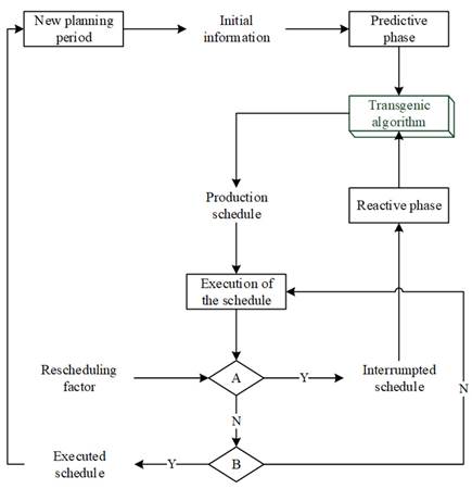
The corresponding integration of the algorithm with the manufacturing environment leads to the following diagram, which represents the utility and operation of the algorithm within said environment.
As seen in Fig. 5, the proposed algorithm is integrated into the manufacturing environment both in the predictive and reactive phase. An initial production timetable is obtained for the transgenic algorithm. Then, said timetable is executed, and decisor A defines whether a rescheduling factor is needed. If this is the case, then the timetable is interrupted and enters the reactive phase to be repaired by the transgenic algorithm. Otherwise, decisor B defines whether the timetable has been completely executed. The timetable is then deemed to be executed, and a new rescheduling period begins. Otherwise, the timetable continues its execution.
Results
In order to assess the performance of the proposed algorithm, this study has been divided into two sections: the first one details the experimentation carried out with the transgenic algorithm in the predictive phase, and the second section involves testing the algorithm in the reactive phase.
3.1. Predictive phase
As described in the third section, this stage includes the generation of the initial production timetable. In order to solve the JSSP, many techniques have been developed. A study on said techniques can be found in 44. Furthermore, these techniques have been tested with comparison instances proposed by different authors. In order to validate the performance of the transgenic algorithm, we selected some alternatives, such as the ones proposed by 45)-(49, and 50.
The results shown below were obtained with the parameterization described in Table VII. Said parameters were set upon the basis of factorial experiments, which are not described in this article in order to avoid content saturation.
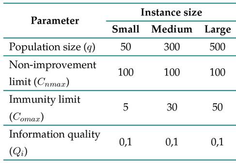
The above-presented parameters have been defined for all three instance sizes: a small instance contains between 36 and 75 operations, a medium instance between 100 and 200, and a large instance between 225 and 400 operations.
Table VIIIsummarizes the results obtained for the selected instances. These instances are assessed in terms of performance compared to makespan. Hence, the BK field yields the best value according to the literature for each instance (some are consistent with optimal values). The BF field states the best value found by the proposed algorithm. The GAP field represents the relative difference of BF compared to BK in percentage form: GAP = 100 × (BF − BK)/BK. The two following fields correspond to the average makespan and its standard deviation obtained for five replicas of the algorithm with the instance.
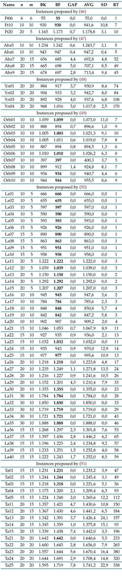
The last field corresponds to the average execution time in seconds. The BF values in bold show that the proposed algorithm has found the BK. The algorithm was implemented in MATLAB. These results were obtained using a computer with an Intel Core i5-8300H @4.0 Ghz and 8GB RAM.
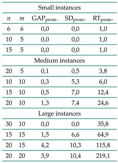
Table IXsummarizes the results obtained after applying the transgenic algorithm to the comparison instances. The average values obtained for the n × m settings are shown. In general, the algorithm performs well in the predictive phase, delivering the best possible values for 52 % of the selected instances and similar values for the remaining instances. These values, on average, do not surpass 1,3 % in the differences for medium instances and 4,2 % for large ones. The algorithm is fairly consistent since the standard deviation is acceptable. Regarding the average execution time, the obtained values are below the minute, except for the last three settings in the set of large instances.
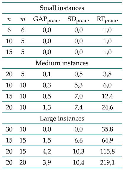
On the other hand, it can be observed that the algorithm’s performance slightly deteriorates as the complexity of the instances increases, i.e., when there are more operations to process. Once the algorithm had displayed commendable performance in terms of average gap, standard deviation, and execution time for the three identified sets of instances, its performance in the reactive phase was tested.
3.2. Reactive phase
Once the initial production timetable is derived from the predictive phase, rescheduling factors will occur at different times of the execution. In this sense, a set of experiments was designed to validate the performance of the algorithm in comparison with the genetic algorithm, an essential reference in evolutionary algorithms. This technique has been used in a wide range of combinatory problems, as mentioned in previous sections. An application of genetic algorithms for operation scheduling and rescheduling can be consulted in 19.
First, given that there are many rescheduling factors, one factor is chosen for each class. It is worth mentioning that, although only one is chosen, the entire class can be solved by the algorithm with a similar procedure. The algorithm can process any of the 17 identified factors. In general, the experiments were designed in terms of the following factors and levels:
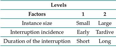
Given the previous factors and levels, a 2 k factorial design was established, with k = 3, corresponding to the number of factors. This setting offers a total of eight treatments, which are detailed in Table XI:
In general, a set of instances were chosen for each class in the predictive phase, in order to design different scenarios. Ten scenarios were built for each treatment, and five replicas were analyzed for each scenario. Regarding the specific values of the levels of each factor, instances with n × m configurations containing 100 operations were considered as small, and those with 400 operations as large. The early incidence includes a random point between 20 and 40 % of the instance makespan. The tardive instance is located between 60 and 80 % of the makespan. Lastly, a short duration corresponds to 40 % of the maximum processing time among all instance operations, and a long duration corresponds to 160 % of the same parameter.
After clarifying the structure of the experiments, the most relevant sections of the genetic algorithm design are presented, with Eq. (6) serving as a reference point to establish the comparison with the transgenic algorithm.

where C max corresponds to the original timetable makespan, and Cm∗ ax corresponds to the makespan of the repaired timetable. The value of E represents the efficiency level obtained for the new timetable in percentage form. A higher value of E means a higher efficiency of the initial timetable.
The stability of the timetable refers to the deviation of the repaired timetable when compared to the initial one 52. It can be measured by calculating the average differences between the starting times of the repaired and initial timetables. Its calculation is obtained via Eq. (7):

where r ij is the starting time of operation O ij in the initial timetable, and ri∗j is the starting time of the same operation in the repaired timetable. R is the set of remaining operations to be processed from the time instant at which the rescheduling factor appears. Lastly, ρ(R) refers to the cardinality of set R.
On another note, the transgenic algorithm for the reactive phase encompasses what is known as the stability factor, which enables the planning staffer to establish a share of operations in R that need to maintain the same sequence as the initial timetable. Hence, the nervousness of the system can be mitigated 3. In this study, the stability factor was determined based on an additional experiment design, carried out with the same factors and levels presented in Table X
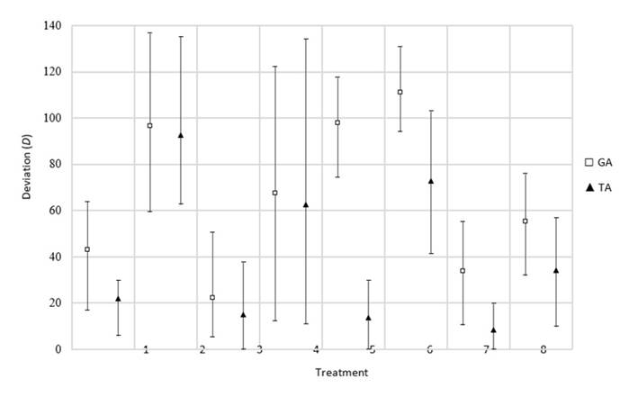
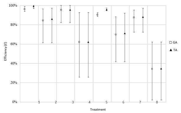
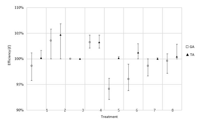
The efficiency (E) and stability (D) results for both algorithms are presented in this section, for each class of rescheduling factor and for each treatment. They are presented in the form of charts that contain the data regarding the minimum, maximum, and average of the performance metrics obtained for the genetic algorithm (GA) and the transgenic algorithm (TA).
In Fig. 6, the performance of the TA in terms of efficiency is equal or superior to that of the GA.
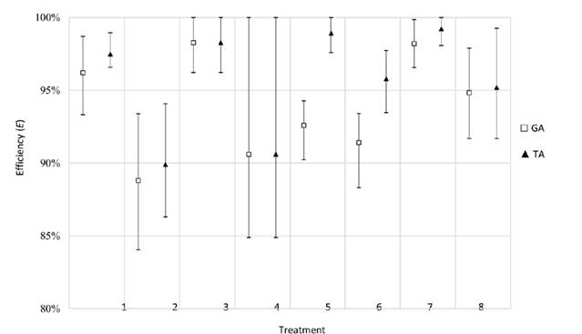
Furthermore, the proposed algorithm exhibits an efficiency close to 100 % when the interruption is short.
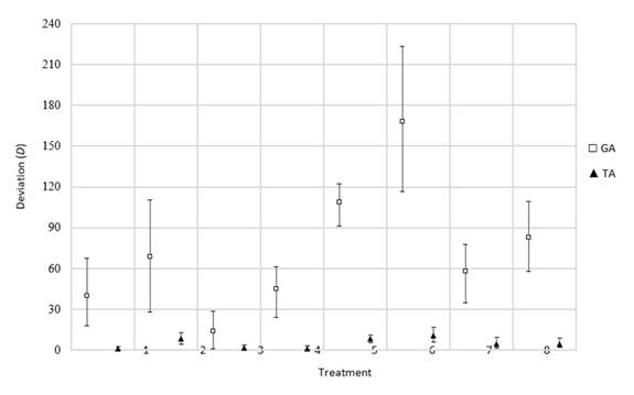
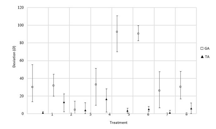
As for the deviation, a better performance is obtained, surpassing the GA in all treatments (Fig. 7). Additionally, the TA performs better in the treatments where the instance is large. One particular case regarding the performance differences between the two algorithms corresponds to treatment 5, where the GA has difficulties with delivering a less deviated schedule than the original one.
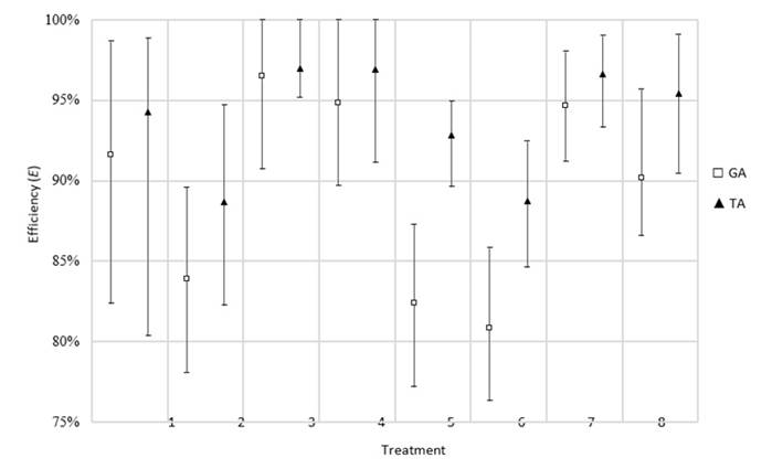
Class II: variation in processing time (7)
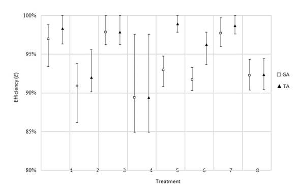
In this set of treatments, a behavior similar to that of the previous rescheduling factor is observed (Fig. 8). This could indicate that these two classes have the same effects on the interrupted timetable. Another interesting fact is that treatment 4 shows a wide range of results, including the lowest performance. This could be explained by the fact that the worst scenario involves a small instance with the greatest variation in processing times for some operations at a final moment (tardive) of the timetable’s execution. The combination of these factors in said levels can lead to a low action range for these algorithms, since there are not many remaining operations that can be rescheduled to compensate for these effects.
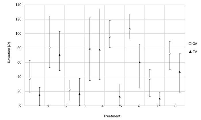
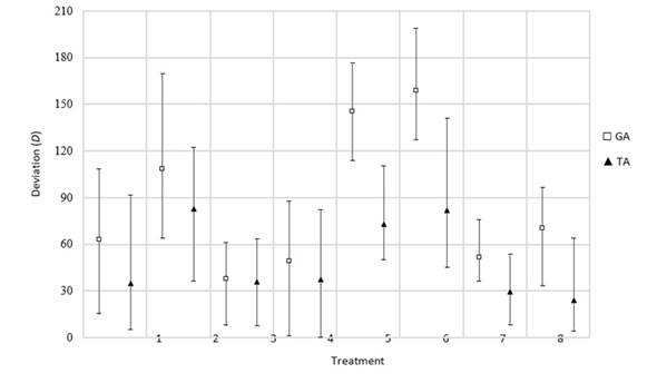
In terms of deviation, a better performance is seen once again, surpassing the GA in all treatments. Additionally. The TA shows a better performance in treatments with large instances. A particular case regarding the difference in performance between both algorithms corresponds to treatment 5 where the genetic method seems to have issues with delivering a timetable that is less deviated than the original one.
Regarding the deviation of the timetables, the same behavior of the previous class is evidenced (Fig. 9). Furthermore, it would seem that the interruption incidence factor had no effect in the deviation of the resulting timetables. It is key to acknowledge that, in this class, the deviations of treatments with short interruptions do not exceed 20 units of time.
This leads to the results shown in Fig. 10. The performance of both algorithms is more even than in previous classes. Hence, a generalized behavior can be evidenced, indicating that long duration is the level that most affects the variability results.
In terms of the deviation of the resulting timetables, the TA shows significantly superior results (Fig. 11). These results could be revealing that the initial timetable has not been able to ‘absorb’ the new job order and has remained almost intact. Thus, the processing of the new order has been delayed for the end. This implies that the efficiency values for this class are not related to the operativity of the algorithms, but with the effect of including a new job after the timetable has begun its execution and, in the worst cases, when it is close to conclusion. Hence, this type of interruption can be handled using the periodic scheduling policy that allows putting the new job order on hold and including it in the next planning period. This ensures an efficient use of productive resources.
In this class, given that there is a priority shift in one of the jobs, the interruption duration factor is analog to the number of remaining operations of the urgent job. This means that the duration factor is represented, in the first level, by the job with less remaining operations when the interruption point takes place. The opposite occurs in the second level.
The results obtained for the efficiency metric reveal that the TA has a superior performance (Fig. 12). The average value of this metric in all treatments surpasses 88 %. Furthermore, the most influential factor is the number of operations. When the urgent job has a higher number of remaining operations to be processed, efficiency is affected.
The algorithm once again yields superior results, exhibiting an efficiency equal or over 100 % in all treatments. The most influential factor is the number of remaining operations for the canceled job. Higher values of this parameter translate into a higher efficiency, as the capacity of resources is slightly relieved.
Regarding the deviation of the obtained timetables, this metric is sensitive to the interruption incidence factor (Fig. 13). When the interruption is early, the stability of the timetable decreases.
Furthermore, this effect is amplified when the urgent job has more operations yet to be processed.
For this class, the interruption duration factor was approached as in the previous class. In this type of interruption, the algorithms handle the elimination of scheduled jobs in the timetable. Hence, the makespan after the elimination of these operations can become lower than the initial one. Fig. 14shows that the values surpass 100 % while maintaining consistency in terms of efficiency.
Once again, the TA demonstrates superior results, indicating an efficiency of 100 % or higher in all treatments. The most influential factor is the number of remaining operations from the canceled job. A higher number of remaining operations leads to greater efficiency, as resource capacity is slightly relaxed.
The resulting deviation validates the performance of the TA, as shown in Fig. 15. There is a variability in the results, which is significantly reduced in various treatments. In general, the algorithm outperforms the GA, offering better results in 65 % of the treatments in terms of efficiency and in 98 % of the treatments in terms of stability. The percentage of remaining treatments for both metrics reveal similar performances for both algorithms.
The average efficiency of the TA is 2,3 % higher than that of the GA. The highest difference in performance is observed in class IV, with an efficiency 4,4 % higher on average when compared to the GA. In terms of the stability metric, the TA shows a standard deviation of 28 units, while the GA deviates by 67 units, thus proving that the former is a complete regeneration method that mitigates the nervousness to a greater extent than the latter.
Lastly, the efficiency and stability of a timetable can be conflictive performance metrics, so the person in charge of planning will have to make swift decisions, seeking to obtain a balanced productive system.
Conclusions
This study focused on developing a computational algorithm to facilitate the job of the people in charge of scheduling production in manufacturing environments. Hence, the theoretical point of view was defined as the starting point in the definition of the Job Shop Scheduling Problem (JSSP).
Given the existing gap between theoretical models and real manufacturing environments, the appearance of unexpected events was included, as they alter the execution of timetables. This sought to provide the proposed algorithm with a more realistic scope. In this sense, a rescheduling framework was selected, which was used to define the Job Shop Rescheduling Problem (JSRP) approach.
Given the increasing complexity entailed by the addition of the aforementioned elements, an algorithm based on transgenic computing was proposed. It was developed while seeking to deliver high-quality production timetables in terms of efficiency and stability.
The performance of the algorithm was validated in both the predictive and the reactive phase. In the predictive phase, a set of well-known instances in JSSP literature were selected. The algorithm performed well, reaching the best-known value in 52 % of the selected instances and similar values for the remaining ones. On average, these values do not exceed 1,3 % of the difference for medium instances and 4,2 % for large instances. Furthermore, as the instance size grows larger, the performance of the algorithm progressively declines. Therefore, the algorithm is not recommended for instances with more than 400 operations, i.e., if similar performance levels are desired.
Regarding the reactive phase, the performance of the transgenic algorithm (TA) was compared to that of the genetic algorithm (GA). The former outperformed the latter, with better results in 65 % of treatments in terms of efficiency and 98 % of treatments in terms of stability. The percentage of remaining treatments for both metrics reveal similar performance levels for both algorithms.
Future work
Given the structure of TAs, there is a possibility that more complex agents can be designed, seeking to improve the performance of the algorithm in instances of higher complexity. On the other hand, the performance of the tool can be more comprehensively validated through a simulation-based study, even with the implementation in a real manufacturing environment.
Finally, given the scope of this work, which is limited to the design and validation of the TA applied to the JSRP, said algorithm could be integrated into real manufacturing environments through the design of a graphical user interface

