


 English (pdf)
 Article in xml format
 Article references
 Send this article by e-mail
 Cited by SciELO
  Cited by Google
  Similars in
SciELO
Similars in
SciELO  Similars in Google
 Permalink
1. Introduction
When simulation models evaluate the performance of supply chains, it is common to look at performance measures, such as cost (including inventory and operating costs) and customer responsiveness (including stock-out probability and fill rate) [1]. These approaches overlook customer (dis)satisfaction behaviors that affect future demand, such as the probability of future purchases and the effects of word-of-mouth in current and potential customers [2,3]. As a consequence, a complete view of the business performance is lacking, particularly when the business environment is repetitive (i.e., future purchases of the same customer are expected and desirable) and competitive (i.e., the customer can easily switch to another provider).
Performance measures based on the customer lifetime value (CLV) might fill this gap. CLV includes a conjoint valuation of customers’ past purchases and expected future purchases due to a sense of loyalty to the company. Loyalty, in turn, can be influenced by the degree of service promise fulfillment by the company in the past [4].
When assessing service promise fulfillment, supply-chain simulation models do not usually address the effects of worker unpunctuality on delivery lateness. Furthermore, we were unable to find a previous simulation study that included customer psychological tolerance to lateness. The inclusion of both phenomena enhances the external validity of the simulation and its usefulness in decision-making without significantly increasing the computational effort.
The aim of this work was to develop a simulation framework in which customer behaviors due to (dis)satisfaction might help to evaluate supply chain performance based on CLV. We also included worker unpunctuality and customer tolerance to delivery lateness as possible moderators within the aforementioned supply chain environment. We expect to produce a simulation model that will help to fill the gap between operations and marketing, leading to a more comprehensive decision support tool in the supply chain.
2. Theoretical background
2.1 Customer lifetime value in supply chain and simulation
Usually, CLV research has focused on attracting, retaining and generating value based on customer loyalty, not on analyzing their impact in the supply chain [5]. Studies on operations research and supply chain, the impact of which is measured through a CLV measure, such as customer satisfaction, loyalty or switching behavior, are hard to find. Several studies claim to measure customer satisfaction, but they do perform that measurement indirectly through service levels or queue performance, such as in [6-8]. Recently, some studies have included basic CLV measures in operations decisions, stressing the need for a more comprehensive vision of metrics between operations and customer satisfaction [9]. Niraj et al. [10] showed the difficulties of estimating CLVs at different stages of the supply chain.
Regarding the specific field of simulation, a review on agent-based simulation in marketing has showed that links with supply restrictions are usually not considered and that word-of- mouth analysis will be beneficial when included in simulation approaches [11]. Among the few manuscripts connecting simulation and CLV, the early work of Ackere et al. [12] applied Monte Carlo simulations to evaluate customer reaction in a waiting line in the long term, although the model was deterministic. Hara et al. [13] modeled the lead time for customer satisfaction using a customer satisfaction index, but the model did not allow for repeated consumption. Switching behavior has also been modeled for supply chains in a competitive environment with a focus on combined contracts [14]. Finally, [15] analyzed mid-term profit for returning customers using a hybrid of agent-based and events simulation to find equilibrium points, but did not address supply chain disturbances. All of the reviewed manuscripts worked with customer satisfaction or switching measures rather than with a unified CLTV measure.
A suitable model of for measuring CLV in a supply chain was recently developed by Tukel and Dixit [4]. In this model, the CLV of a customer j is evaluated as follows:

PPC j is the profit contribution of past purchases from customer j
FPC j is the forecasted contribution of future purchases from customer j
Ll j is a loyalty index of customer j
PPC j and FPC j are calculated as follows:


where pit is the profit contribution of product i in time period t and qit is the total quantity of product i sold to customer j in time period t. Fpit and Fqit are the forecasted profit contributions of product i in time period t and the forecasted total quantity of product i sold to customer j in time period t, respectively.
2.2 Worker unpunctuality and unpunctuality tolerance
Worker unpunctuality has been primarily researched in psychology. Porter & Steers [16] noted several psychological characteristics that influence unpunctuality. Ferris et al. [17] found a relationship among unpunctuality, anxiety and absentees. A similar work [18] found relationships of unpunctuality and several labor and psychological factors, including work satisfaction and alcoholism. A possible distribution function for worker unpunctuality is a power-law function [19], in which a large portion of delays are short, but extreme delays are still possible.
Therefore, it is not surprising that unpunctuality perception differs among cultures. For instance, Brazilian and United States workers differ in their perception of unpunctuality and, as a consequence, in their tolerance to unpunctuality [20]. Particularly important for the present study, tolerance to unpunctuality - called On Time Window (OTW) - has been found to be highly negatively correlated with the Human Development Index [21].
2.3 Customer behavior after (dis)satisfaction
Known models of responses to dissatisfaction have found three different responses from dissatisfied customers: a) ending the relationship with the company or reducing purchasing frequency, b) complaining, or c) maintaining their loyalty to the company in spite of their dissatisfaction [22]. Another possible behavior after dissatisfaction is negative word of mouth (NWOM), which involves communicating dissatisfaction to others, without including the service provider [23]. As a consequence of NWOM, organizations might suffer a loss of credibility, which in turn, affects their reputation within the market and significantly reduces their profits [24]. In the case of satisfied service, there can also be positive word of mouth (PWOM) [25]. The effect sizes of word of mouth are difficult to determine. Some studies have shown that word of mouth can account for up to 50% of sales [26]. A cross-industry study, ranging from restaurants to technology industries, showed that the force of PWOM is usually greater than the force of NWOM for purchasing behavior and that it differs across studies; however, the probability of an effective influence due to PWOM did not surpass 50% [27]. A recent meta-analysis also showed that PWOM force was greater than NWOM force, but warned that there was a possible deviation from linearity in the decision making process [28].
To be important to an industry, the above explained customer behaviors need to be exerted in business models in which customer loyalty can affect company results. Particularly, the possibility of a customer expressing (dis)satisfaction through repeated consumption of the products/services of the company and the possibility of a customer switching between providers are of the utmost importance for the CLV effects to be measured. Therefore, it is necessary to emphasize that the developed model is particularly applicable in repetitive and competitive environments.
Several simulation models have addressed the issue of customer behaviors as agents and their impact on operations performance [29] or marketing research [11]. However, to the best of our knowledge, none of these simulation models have addressed this specific issue in the supply chain through CLV measures or by taking into account the issue of worker unpunctuality.
3. Simulation conceptual model
We decided to work with a hybrid model (i.e., agent-based and discrete-event based). Agent- based simulation allowed us to model behavior at the customer level with detail; on the other hand, simulation at the service level was facilitated by well-known discrete-event simulations. As a consequence, properties emerged from the lower (customer) level to the higher (service) level [30].
There is an initial set P of potential customers. From them, a subset Pa of potential costumers becomes the actual customers at the beginning time t and places orders with the company. A complementary subset Pe of customers remains potential customers. Each customer belonging to Pa is assigned a frequency intention of purchase Fi that depends on its loyalty Li. All potential customers have the same tolerance to delay OTW (Figure 1). These behaviors are modeled through agent-based simulation.

The company delivers a service promise S, which is the time when it expects to deliver the product with a confidence level. Then, using discrete-event based simulation, the supply chain makes the product, spending time D to deliver the product, which is the sum of the entire time of the supply chain process (supplier, producer and distributor), including possible delays due to worker unpunctuality. This unpunctuality is governed by a probability distribution law U.
For each customer of Pa, one of the following might happen, as modeled through agent-based simulation:
D is below or equal to S. The customer is satisfied and therefore performs the following two actions: a) The customer sends PWOM messages to k customers of Pe, with an effectivity probability PWOMe. If the message is effective, a new customer passes from Pe to Pa. b) The customer updates their loyalty L according to their recent experience with the company, remaining a customer of Pa with an updated frequency Fi.
D is above S, but below or equal to the S plus customer tolerance window to delays (OTW). The customer is temporarily dissatisfied and, as a result, sends NWOM messages to l customers of Pa, with an effectivity probability NWOMe. If the message is effective, a customer passes from Pa to Pe.
D is above S + OTW. The customer is dissatisfied and therefore performs the following two actions: a) The customer sends NWOM messages to m customers of Pa, with n effectivity probability NWOMe. If the message is effective, a customer passes from Pa to Pe. b) The customer updates their loyalty Li according to their recent experience with the company. If their loyalty is below a loyalty threshold Lh, the customer passes from Pa to Pe. If the customer loyalty is above Lh, the customer continues to purchase with an updated frequency Fi.
4. Experimental design and results
The system under study in the simulation was a make-to-order supply chain with two suppliers, two sequential production processes, and a single distributor.
An experimental design of 33 * 4 was proposed to evaluate the effects of different values of PWOMe, NWOMe, OTW and U on the percentage of switching customers, number of sales per customer, customer loyalty and percentage of potential market reached.
The levels of the effectiveness of PWOMe and NWOMe were chosen from the cross-industry study of East et al. [27]. Three values of effectiveness were selected for PWOMe and NWOMe, the highest (39% and 20%), the average (20% and 11%) and the lowest (1% and 3%), across industries. OTW was calculated based on its relationship with Human Development Index described by [21]. The United States, Estonia and Colombia were selected as representative of low, medium and high OTW levels (20.8, 26.3 and 32.5 minutes, respectively), respectively, given their position in the Human Development Index of 2014. U (the unpunctuality function) was set to a Pareto distribution according to a field study. This distribution allowed a Pareto rule to be modelled in which short delays account for a high proportion of the total delays and is consistent with the power-law findings in an unpunctuality distribution [19]. The values of the a parameter were selected to match 15 minutes differences according to the research of With et al. [21], including a fourth level for punctuality.
At zero simulation time (t=0), a random number [0,1] was generated to define Pa, the initial fraction of P customers that become current customers. Notice that each customer belonging to Pa starts to purchase depending on its frequency of purchase Fi.
Loyalty was initially set for each client as a random number between [Lh,1], and Lh was set to 0.2 because a minimum loyalty is needed to start buying.
According to the literature, loyalty is mainly influenced by two factors: service quality and commitment to the provider [31], also called brand equity. The influence of service quality is usually direct, whereas the influence of brand equity is mediated and indirect [32]. Our model suggests that brand loyalty is tied to past experiences. Therefore, loyalty at time t can be calculated as
Lt = r * 0.6 + Lt-1 * 0.4 (4)
where t represents a cycle of purchase for the customer and r is a binary variable, which is 1 if the customer is finally satisfied and 0 if the customer is dissatisfied. Thus, we weighted service quality as having a higher impact than brand equity.
To avoid a system that is too idle or too busy, the relationship between the number of potential customers and frequency of purchase was kept constant.
The values of k, l and m (the number of word-of-mouth messages) were set at eight to attempt to simulate a basic family and some friends.
The following validation tests were conducted: a) A supply chain without independent variables effects was tested to deliver products within the expected values according to the assigned probability functions; b) the values of the independent variables were set to the middle value, and the results were tested for face validity; c) each single independent variable parameter was set to their highest value and the other independent variables were set to zero to produce the expected main effects for each variable; and d) the results of the dependent variables were graphed against time to graphically determine the appropriate simulation length for the steady state to be reached.
At the simulation production stage, we performed 87 replications for each of the 108 treatments, all of which with a length of 10,000 time units. The number of replications was calculated based on a middle size effect.
To analyze the experiment, ANOVAs were performed on each dependent variable. The percentage of switching customers and the percentage of potential market reached were transformed with the square root, as suggested by Jaeger [33]. Given that the ANOVA assumptions did not hold, a confirmatory Kruskal-Wallis test were conducted. To estimate the effect sizes, Tukey DHS tests were conducted.
The main effects results, with their directions, are shown in Table 1. Lower unpunctuality levels led to better results for the company (a lower percentage of switching customers, higher sales per customer, higher loyalty, and higher market reached). The effects ranged from a 4.4% to 6.3% increase, on average, of the market reached, 1.5 to 4.5 additional average purchases per client and from a 9% to 15% average loyalty increase. Although the impact of delays on satisfaction has been measured [34], the effects on CLTV measures are hard to measure due to its long-term nature, and this manuscript is a first step towards the measuring these impacts.
Table 1 Significant effects and directions of independent variables in CLV metrics

Source: Authors’ own creation
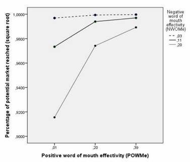
As expected, higher PWOMe led to better results for the company, whereas higher values of NWOMe led to poorer results. However, there was a strong interaction between PWOMe and NWOMe. Previous research has measured WOMe effects in isolation. As a consequence, our results represent a first attempt to explain the better interwoven and non-linear relationships between PWOMe and NWOMe suggested by [28].
Figure 2 shows this interaction effect for the percentage of the market reached, but the same effect held for all CLV measures. When there is a low PWOMe effectivity, changes in NWOMe effectivity have a specific impact on CLV measures. As long as the PWOMe effectivity increases, the effects of NWOMe are reduced and almost disappear (Figure 2). Thus, a smoothing effect of PWOMe over NWOMe was observed.
Source: Authors’ own creation
Figure 2 Interaction between NWOMe and PWOMe for the percentage of market reached
Note that OTW had no significant effects on the dependent variables. It seems that the inherent variability of the entire supply chain took on the fluctuations generated by worker unpunctuality.
5. Conclusions
We developed a scalable and flexible model that helps to assess the impact of customer and worker behaviors on CLV metrics. This model helps to improve mid- and-long term analyses of industries in which the competitive environment is tough and a high frequency of customer purchase is important to succeed. Our expectation is that this tool might enlighten business decision-making.
From the proposed variables that affect CLV, the relationships between PWOM and NWOM are important to consider. It is possible that moderator effects between these factors might help to explain some literature findings, particularly the non-linear relationships between PWOM, NWOM and CLV measures. It is important to note that PWOM counteracts the effects of NWOM only until a certain level. Beyond this level, delays of the supply chain must be fixed through operational research and operational strategies.
The assumptions made are important to understand the limitations of the present work. Given that a single-level supply chain was modeled, our results are not generalizable to more sophisticated supply chains. Other possible customer reactions to delays on delivery were not taken into account. Moreover, different reactions of different segments clients were not modeled. The results are only valid for competitive high purchase frequency environments with single-level supply chains, such as the food retail industry or clothing industry. However, we believe that our results open an avenue of research that combines hybrid and discrete-event simulations, allowing customer level psychological phenomena to be simultaneously consider along with the operations level performance and modeling.
Further developments will include developing tools for make-to-stock supply chains, calculating a more precise OTW for specific industries, developing agents for different market segments and analyzing thoroughly warming times.

