


 English (pdf)
 Article in xml format
 Article references
 Send this article by e-mail
 Cited by SciELO
  Cited by Google
  Similars in
SciELO
Similars in
SciELO  Similars in Google
 Permalink
1. INTRODUCTION
In contrast to the classical generation paradigm, Distributed Generation (DG) employs appropriate technology for small- and medium-scale electricity generation near its consumers [1]. In Colombia, DG is defined as electricity production close to consumption centers and connected to a Local Distribution System (LDS) [2]. In 2014, the Congress of Colombia [2] determined that the capacity of distributed generation would be defined according to the dimension of the system to which it will be connected, complying with the terms of the connection code and the other provisions that the Regulatory Commission of Energy and Gas (CREG in Spanish) establishes for that purpose. In 2018, the CREG regulated the activities of small-scale self-generation and distributed generation in the National Interconnected System in Resolution 030-2018 [3]. In [3], the CREG stablished two types of “auto-generators” who use generation systems, such as DG, to produce electrical energy mainly to meet their own needs. The first type is large-scale auto-generators who have an installed power exceeding 1 MW. The second type is small-scale auto-generators who have an installed power equal to or lower than 1MW [3].
With the increase in electricity demand in the country, the environmental challenges of generation systems have also increased. The Government’s interest in supporting the implementation of new generation technologies has led to economic decisions that help to motivate the industrial and commercial sectors to implement systems to generate electricity from Non-Conventional Energy Sources (FNCE in Spanish) and Non-Conventional Renewable Energy Sources (FNCER in Spanish), as defined in [2]. Renewable sources and other distributed resources (including storage, smart appliances, PHEVs with vehicle-to-grid capability, and micro-grids) offer a unique opportunity to transform the distribution system into an active and controllable resource [4]. Electrical networks are designed to operate in a unidirectional power flow scenario, but nowadays electrical systems must also be able to integrate active actors that are not dispatchable (such as Renewable Energy Sources, RES) along with components that may partially change their role (for instance, active users with Demand Side Management, DSM, installations) [5]. In this new generation paradigm, companies that operate distribution networks are interested in the impact of these DG connections on the environment and low-voltage networks [6], [7].
To integrate new generation systems into electrical grids, a power-flow study should be conducted in the area of influence in order to verify the system before and after the changes to the grid. The electricity production of renewable sources varies with solar radiation or wind speed, making power generation a function of time. Such variation requires the use of quasi-dynamic simulation, a time-varying load-flow calculation tool to perform load-flow simulations during a certain time (in this case, a twenty-four-hour period) in the different nodes of an electric power system. Different authors point out that quasi-dynamic methods not only improve the fidelity of the simulation in the general process compared with quasi-static methods, but also reduce the processing time of the dynamic simulations [8], [9], [10], [11] y [12].
2. SIMULATION OF THE IEEE 13-NODE SYSTEM WITH DISTRIBUTED GENERATION
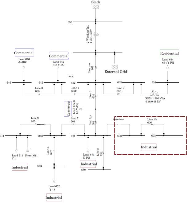
The IEEE 13-node test system is an electric network with a voltage level of 4.16 kV that represents a small and highly-charged radial distribution system [13]. The IEEE 13 Node Test Feeder has the following characteristics:
Small electric network with very high chargeability.
Voltage regulator in the substation (three single-phase units connected in Y).
Presence of aerial and underground lines in the system.
Capacitor banks and a distribution transformer 4.16 / 0.48 kV.
Unbalanced loads: spot and distributed.
2.1 Load modifications
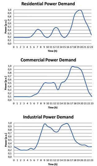
For each load in the IEEE 13-node system, a daily demand curve was modeled based on the power demand curves of the Colombian residential, commercial, and industrial sectors [14]. Industrial nodes were included with DG since they represent potential users that could have the economic resources to acquire and generate electricity independently, although industries could obtain better profits from eventual discounts and assistance offered by the Colombian government, making self-generation more attractive for investors.
The residential curve was incorporated into a low-voltage node (480 V), and the commercial curves were incorporated into the Distributed Load and two other nodes, close to the connection point of the local distribution system. The characteristics of the nodes are detailed in Table 1.

2.1.1 Modeling the Distributed Generation Systems
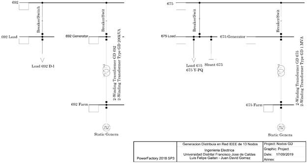
The new Distributed Generators (DGs) in the IEEE 13-node system (small-scale auto-generators, AGPE in Spanish, installed at two industrial nodes) were modeled with the Static Generator tool in DIgSILENT® Powerfactory software, which models DG technologies connected to a network through an inverter [15], [16].
The spot-type load in the original power system was taken as the reference value for the characteristics of these generators, such as active and apparent power. Furthermore, the DGs were simulated as 0.9 inductive. Fig. 1 and Fig. 2, show how the load and the new generators were connected in the IEEE 13-node system. The power values of the new generators included are listed in Table 2.

2.1.2 Modeling the transformer for the alternative generators
In the new DG zone, the simulation needs a special transformer to change the voltage level between the new generation system (Static Generator, DG node) and the node with the system connection point, where the original load is installed. A Breaker/Switch is used to control the connection of the DG node with the AGPE node. The losses of the new transformers are about 3 %, and their star connection is in neutral zero (YN-YN-0). Other values are the default values generated by DIgSILENT® Powerfactory.
2.2 Simulation scenarios
To identify changes in the LDS with the new DG nodes, three simulation scenarios were established:
Source: Authors.
Fig. 2 Simulation of the IEEE 13-node system with loads modified based on the behavior of the Colombian
2.2.1 Conventional scenario
In this operation scenario, node 650 is the only power source of the electrical network. The industrial loads with DG systems are not using their auto-generation systems.
2.2.2 Distributed Generation scenario, “Noon Peak”
In this operation scenario, the electrical network has the new DG sources. Industrial nodes 675 and 692 have their DG systems operating. A previous research investigation indicates that the maximum power injection of the new generation units should be guaranteed during grid analysis [17]. Following that recommendation, the DG systems are set to their full generation capacity. The DG systems begin their power dispatch at 10:00:00 hours and end at 14:00:00, responding to the noon peak in the typical demand load curve of the country, as can be seen in Fig. 3. and Table 3. shows the load modifications in the scenarios.
Source: Authors.
Fig. 3 Scheme of the modified IEEE 13-node system with distributed generation at nodes 692 and 675

2.2.3 Distributed Generation scenario, “Night Peak”
Adopting the same dispatch philosophy, in this scenario, the DG systems begin their power dispatch at 18:00:00 hours and end at 22:00:00, attending to the biggest peak of the daily demand load curve of the country, as shown in Fig. 1.
3. “QUASI-DYNAMIC” SIMULATION
DigSILENT® Powerfactory offers quasi-dynamic simulation for the execution of medium- to long-term electrical studies. This type of simulation performs multiple load-flow calculations with user-defined time-step sizes. The tool is focused on planning studies in which long-term load and generation profiles are defined, and network development is modelled using variations and expansion stages [18].
One of the advantages of this simulation strategy is that it offers a faster way to complete the calculations because it does not require to solve all the mathematical requirements, which means a faster computation process with fewer hardware resources. Other works [16], [19], [20], indicate that the quasi-dynamic approach achieves better fidelity than other methods, such as the quasi-static [21], [22], [23], [16]. For that reason, quasi-dynamic simulations are used in different fields like physics, seismology, and electronic applications [8], [9], [19].
Quasi-dynamic simulations have been employed in electrical system studies into topics like power interruption devices [10], photovoltaic systems [11], [12], heating systems [19], [20], training simulators [21], and distribution systems studies [4].
In [24] and [25], the quasi-dynamic tool is used to analyze the behavior of two transmission grids that serve industrial customers after an Economic Dispatch Optimization of the traditional and new DGs included in the power system. The grids are the IEEE 14-node system, which is a representation of an electrical transmission system in the Mid-Western USA of 1962; and, on the other hand, the IEEE 30-Bus Test Case, which represents a portion of the American Electric Power System in the Midwestern USA as of December, 1961.
In this work, the tool is used to analyze a distribution system with different kinds of customers in order to determine the behavior and changes of the grid when some nodes in the system include DG systems in accordance with some aspects of the most recent CREG regulation [3].
With the modification of the loads, each node in the system has a different power demand minute by minute. This new behavior varies according to the type of demand analyzed in each scenario. Moreover, because in the two proposed scenarios the network has new generation nodes, it is necessary to study the behavior of the system before the introduction of these new generators in order to find possible problems in its operation.
To determine the performance of the system with distributed generation sources, in this study case, the load flows are calculated every minute for 24 hours in order to identify changes in some of the electric network variables.
Additionally, in the simulation, the losses in transformers and system lines are calculated in the conventional and the two DG scenarios. To better visualize the simulation results, the IEEE 13-node system was divided into two zones: Zone 1 contains nodes 646, 645, 632, 633, 634, and 671; and Zone 2, nodes 611, 684, 692, 675, 652, and 680. The most significant variations are analyzed below.
3.1 Variations in voltage profile
The voltage variations are illustrated in Fig. 4. In Zone 2, there is just a small increase in the voltage level of node 611 (red line) in the two DG scenarios, depending on the operation of the new DGs in the systems. In the other nodes, the system does not exhibit important voltage level changes, only a small increase at different hours, depending on the operation times of the DGs.

The graphs show small changes in the voltage level during the voltage peak of each DG scenario. Furthermore, the three scenarios produce the same maximum and minimum voltage levels.
Fig. 4 indicates that the operation of the DGs in the system does not represent significant changes in the system voltage profiles. The figures in this section are Voltage [p.u.] vs. Time [hours] curves.
3.2 Variations in active power profile
Fig. 5 and Fig. 6 illustrate the variations in the active power profiles in the two zones of the LDS. The modification implemented in the system produces significant changes in the active power levels. In the two zones, there is a significant decrease in the voltage level of nodes 632, 671, 675, and 692 in both DG scenarios.

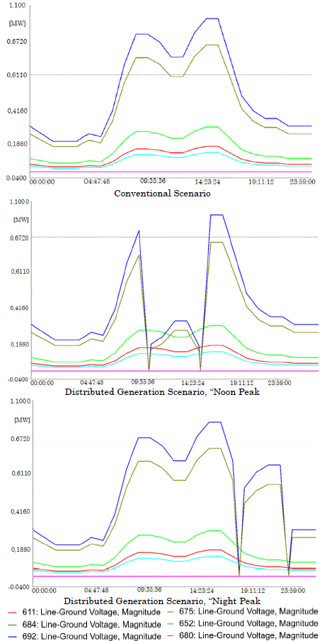
Fig. 5 shows how nodes 632 and 671 change their active power levels during the DG operation. These nodes are important because they connect the industrial nodes of the grid. Their power level decrease is the consequence of the low power demand at the DG nodes, which now are generation nodes of the LDS.
Fig. 6 illustrates how nodes 675 and 692 nodes change their active power levels during the activation of the DG systems. In the conventional scenario, two decreases can be seen in the power peak: one small close to 13:00 hours and an important one after 18:00 hours. This phenomenon produces an increase in the active power present in the DG nodes because, during those time periods, the power demand is lower than the generated power. The figures in this section are Active Power [p.u.] vs. Time [hours] curves.
3.3 Variations in reactive power profile
Fig. 7 presents the variations in the reactive power profiles. The new DG nodes do not imply significant changes in the reactive power levels. The reason for these unaffected active power levels is that the DG systems do not deliver reactive power to the grid. The figures in this section are Reactive Power [Mvar] vs. Time [hours] curves.

4. RESULTS AND DISCUSSION
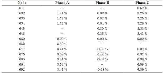
4.1 Voltage variations
The voltage levels of the nodes do not present important changes during the operation of the DGs. Table 4. shows the small differences between the voltage levels of the nodes when the DG systems are operating (DG scenarios) and those in the conventional scenario.
4.2 Variations in distribution line losses
Fig. 8 compares the line losses in the conventional and DG scenarios; and Fig. 9 the line currents in the same scenarios. Table 5. lists the changes in electrical line losses in both scenarios. In this case, the line losses decreased. Due to the implementation of the new generators, the current flow of Line 10 increased from 83 to 181 amperes, which directly affects the losses in that line.

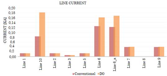

In the Distributed Generation scenario, some line losses decreased up to 107.86 %, but others escalated. In Line 6, losses increased by 99.15 %; in Line 6a, 125.08 %; and in Line 10, 300.11 %. Line 6a is the same Line 6 divided by the distributed load.
Those increases in line losses were caused by the generation units at nodes 695 and 675, but Line 10 was the most affected. The implementation of such generation units caused bidirectional power flows that resulted in greater line losses. If only the demand of the industry is satisfied, losses in the system would decrease.
4.3 Behavior of the transformers
The transformers do not exhibit important changes in their electrical parameters. With the DGs, the transformers of the LDS present a good performance. The distribution transformer shows just a small increase in power losses, 2.4 %, because the current increases on the high-voltage side.
Table 6. shows the percentage of change in transformer parameters on the HV side.

5. CONCLUSIONS
This work analyzed a distribution network with a high-power demand and loads that incorporated Colombian residential, commercial, and industrial demand curves. Two nodes in this study case can deliver power to the LDS from their backup generation systems, whose capacity is the same as the load they demand from the system. If the objective of including DG is to address the peaks of the system trying to flatten the energy demand curve, we must make sure that the generation technology is able to operate within the time margins where demand is higher.
DG systems do not produce significant changes in this LDS, but it is necessary to pay special attention to the operation of the DGs because some lines of the system could present high currents. Additionally, the active power levels could be higher when the power demand decreases. The voltage profiles resulting from the quasi-dynamic simulation do not show considerable changes in the behavior of the electrical network when DGs are introduced.
In the Distributed Generation scenarios, the introduction of the DGs into the system represents a 107.8 % increase in line losses. In addition, the currents in Lines 6, 6_a, and 10 rose 61.6 % on average.
In this study case, to avoid problems in the LDS, the switch that separates nodes 692 and 675 from the system should be activated. By doing this, the self-sufficient industry operates in islanded mode, the existing infrastructure of the network is not affected, and the system’s demand for electrical power decreases. If distribution network operators want to use the DG as a new generator in the LDS, they should implement new lines in the network in order to not to affect the normal operation of the system.

