


 English (pdf)
 Article in xml format
 Article references
 Send this article by e-mail
 Cited by SciELO
  Cited by Google
  Similars in
SciELO
Similars in
SciELO  Similars in Google
 Permalink
1. INTRODUCTION
Cocoa beans are the dried and fully fermented seeds from the cacao tree (Theobroma cacao). Although this tree originated in America's rainforests, it is also grown in the tropical areas of Africa and Asia [1], [2] Cocoa constitutes a valuable agricultural commodity for more than 40 million people around the world [3] In addition, the chemical quality attributes of raw cocoa [4] make it highly demanded by the confectionery, aesthetics, and healthcare industries (see Table 1) [5], [6] , [7].

A total of 68 % of the world's cocoa beans come from Africa-the largest cocoa producer worldwide-, while only 17 % are produced by Latin American countries (Brazil, Ecuador, Mexico, Peru, Dominican Republic, and Colombia) [8]. In addition, the best and most expensive quality cocoa, known as premium cocoa (5 % of the world’s cocoa), comes from Latin America [9], [10]. Global cocoa production has increased significantly in recent years, hitting a record of 4.85 million tons in 2019 [11]. However, it has not been enough to meet the world’s demand [12]. For this reason, the International Cocoa Organization (ICCO) has suggested Latin American countries to increase their cocoa exports. To that end, less complicated and faster classification processes must be explored [13], [14]
Nowadays, in most cocoa international markets, the methods employed to classify beans consist of chemical, physical, and sensory analyses that take approximately 26 hours [15]. Additionally, this classification is often carried out with samples, that is, 100 grains per ton, to determine the quality of the load. Said analyses require tasters, technical personnel, specialized equipment, and the destruction of the samples [1], [6]
Moreover, Hyperspectral Image (HSI) acquisition and processing techniques have been increasingly used in food quality control [16] [17], [18], [19], [20]. A hyperspectral image can be represented as a three-dimensional data cube, F∈R (M × N × L ) , where M and N correspond to the spatial dimensions; and L, to the spectral dimension. Each element reflects, absorbs, and emits electromagnetic energy in different magnitudes at each specific wavelength according to its physical and chemical composition [21], [22]. Therefore, two elements with a different composition can be identified or associated through their spectral signatures [23], [24], [25], [26]
Some studies have been conducted in India, Ghana, Peru, and Germany to evaluate the quality parameters of cocoa beans using spectral information [27], [28], [29], [30], [31], [32], [33], [34]. For instance, in [33], the composition and aroma profiles of 26 cocoa beans were assessed using Mass Spectrometry (MS)-fingerprinting and Headspace-Solid Phase Micro-extraction-Gas Chromatography-Mass Spectrometry. As a result, the authors classified the beans into fine flavor cocoa, well-fermented cocoa, and low-quality cocoa. In [27], the fermentation index, pH, and polyphenol content of cocoa beans were calculated. The whole grains were used for the spectral measurements in the near-infrared range, while, for the chemical analysis, they were grounded into a fine powder. According to the results, an accuracy greater than 80 % in the fermentation index and total polyphenols was achieved. In general, these and other studies have followed chemical procedures that, although precise, involve invasive stages and require very specialized personnel; hence, they could not be generalized to all marketable beans.
Recent works have demonstrated that grouping pixels with similar characteristics within an image (called superpixels [35]) before processing HSIs makes it possible to obtain more accurate classification results and reduces the computational cost and time required by supervised classification methods [36], [37], [38], [39]
Specifically, [38] presents a multiscale HSI strategy based on superpixels to classify remote sensing images and obtain results that are up to 3 % more accurate than those provided by classification methods that do not use superpixels. Furthermore, the approach followed in [39] groups the spatial information of a Red, Green, Blue (RGB) image into superpixels and fuses such features with the spectral information of a HSI. The results show that the proposed classification method optimizes the overall accuracy and reduces the computational complexity compared to traditional approaches in which all pixels are used.
Similar results are reported in [36] and [37]. However, the superpixel technique with hyperspectral classification has not yet been used to evaluate, in a noninvasive manner, the classification of cocoa beans.
Therefore, in this study, we propose a noninvasive approach to classify cocoa beans into three categories based on their fermentation level using their hyperspectral images. In particular, the proposed classification method includes the following stages: sample preparation, acquisition of cocoa beans’ spatio-spectral information in the visible and near infrared (350-950 nm) ranges, background subtraction, feature extraction with superpixels, and hyperspectral classification.
The rest of this paper is structured as follows. Section 2 summarizes the stages of the proposed method. Section 3 provides an analysis of the data and presents the results. Section 4 draws some conclusions and outlines some future lines of work.
2. MATERIALS AND METHODS
This section details the proposed classification methodology and the data acquisition process.
2.1 Cocoa Selection
The cocoa beans were harvested in a farm located in the town of Rionegro, Santander, Colombia (7° 15' 51" N, 73° 08' 58" W). These beans were extracted from cocoa pods within the same hectare and then fermented by a local farmer. Experts from the National Cocoa Federation in Colombia selected 30 samples for each of the three fermentation levels: (i) slightly fermented (LF), (ii) correctly fermented (CF), and (iii) highly fermented (HF). In total, 90 cocoa beans were selected.
Afterwards, the beans were evaluated in an optical laboratory and their spectral data were captured using the experimental setup described below. The environmental conditions in the laboratory included a temperature of 23 °C and a humidity of 60 %.
2.2 Experimental Setup
An optical assembly was built in our laboratory to capture hyperspectral images of the cocoa beans. The built testbed is shown in Figure 1. The scene (cocoa beans) was illuminated with a tunable light source (Oriel Instruments, TLS-300 XR) that decomposes the illumination from a halogen light source in its corresponding monochromatic wavelengths, with steps of two nanometers within the spectral range between 350 and 950 nm. Such monochromatic light is propagated through a bifurcated optical fiber (Illumination Technologies, 9145HT dual 6” light line) towards two lamps that illuminate the scene.

A monochromatic sensor (AVT Stingray F-080B) captures the intensity of the light reflected by the cocoa beans (G
ref
(λ)). Each obtained hyperspectral image exhibits 1032 x 776 pixels of spatial resolution (M x N) and 301 spectral bands (L). Also, a white scene (G
inc
(λ)) was acquired to calibrate the hyperspectral information as
 Six beans were organized for each scene, considering the focus and field of vision of the setup. In total, five data cubes were obtained for each of the three fermentation categories, which resulted in 15 spectral images, F∈R
(M × N × L
),
each with six beans of the same category (i.e., a total of 90 cocoa beans captured).
Six beans were organized for each scene, considering the focus and field of vision of the setup. In total, five data cubes were obtained for each of the three fermentation categories, which resulted in 15 spectral images, F∈R
(M × N × L
),
each with six beans of the same category (i.e., a total of 90 cocoa beans captured).
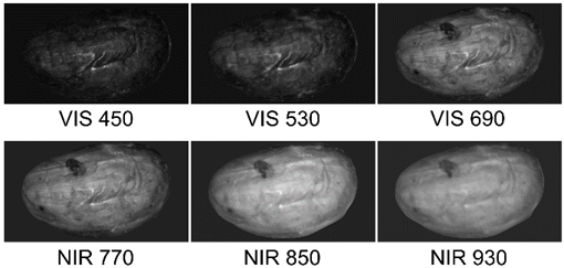
Figure 2 presents six of the 301 spectral bands of one random bean, which were acquired following the proposed setup. In addition, it spectral band includes the spectral range (VIS by visible or NIR by Near-infrared) and wavelength of each band in nanometers. We freely published the spectral images of the 90 cocoa beans on IEEE DataPort [40]. Figure 3 plots the mean spectral responses of the three fermentation categories. After the spectral information of the cocoa beans was obtained, the spectral images were processed.
Source: Authors’ own work.
Figure 2 Examples of some spectral bands captured by the optical assembly for each bean

2.3 Background Subtraction
The first stage in HSI processing consists in identifying and extracting the pixels containing the information of interest, that is, the beans. Since the background of the images is black, a binary mask (D) that identifies the position of the beans was created using thresholding.
Additionally, morphological operations were employed. The values of the pixels in the binary image, D, are adjusted based on the value of other pixels in its neighborhood, such that the binary result (D∈R (M×N) )is a given closed figure (B). The closing operator consists of a dilation operator and an erosion operator. The dilation operator, on the one hand, adds pixels to the boundaries of the objects in the image and is mathematically expressed as (1).

The erosion operator, on the other hand, removes the pixels in the boundaries of the objects and is expressed as (2).

In this study, following the shape of the beans, B is chosen as an oval shape of 200 x 300 pixels. Then, the result of the closing operation is given by (3).

Finally, the binarized image, D, is multiplied with the hyperspectral image, F ∈R M × N × L , of each sample to obtain the reflectance values of the cocoa beans as follows (4):

Where ∘ is the Hadamard product; and
 , the HSI without background information. Figure 4 shows a HSI, F; its binary mask, D, which was obtained with (3); and the respective dataset,
, without background, which was calculated using (4).
, the HSI without background information. Figure 4 shows a HSI, F; its binary mask, D, which was obtained with (3); and the respective dataset,
, without background, which was calculated using (4).

2.4 Feature Extraction
The second stage in the proposed framework involves extracting the classification features from
. Recent works have demonstrated that segmenting spectral information into spatial superpixels reduces the computational cost required by supervised classification methods and increases accuracy [36], [37], [38], [39]. Since traditional superpixel algorithms operate on three-band images (e.g., RGB images), we propose the following to extract the classification features: first, a three-band (RGB) image of the
hyperspectral data cube is extracted. Notice that
is acquired from the range between 350 and 950 nm. Then, from the
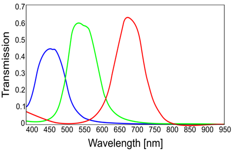
data cube, the spectral bands corresponding to 460, 530, and 670 nm are selected to form a three-band image (R,G,B). The three wavelengths represent the spectral response peaks of the blue, green, and red channels, as shown in Figure. 5.
Source: Adapted from [41]
Figure 5 Theoretical spectral responses of the red, green, and blue channels
Afterwards, a segmentation algorithm is applied to the three-band image to find a superpixel map. For this purpose, we specifically use the well-known Simple Linear Iterative Clustering (SLIC) algorithm [35]
The SLIC algorithm works in the five-dimensional space, where the two coordinates (x, y) correspond to the spatial location of the superpixel and the other three components depict the RGB channels. The input variable of this algorithm is the number of desired superpixels (N spx ). Given N spx , where the approximate size of each superpixel is MN⁄N spx , the SLIC algorithm defines a cluster center at every grid interval, S, as follows (5):

Hence, the algorithm chooses N spx superpixel cluster centers, Cj = [rj, gj, bj, xj yj ] T , with j = [1, N spx ]
The SLIC algorithm assumes that the pixels associated with a cluster lie in a 2S × 2S area around the superpixel center on the (x, y) plane. Therefore, this is the pixel search area near each cluster center. The center is transferred to the lowest gradient position in a 3 × 3 neighborhood to prevent it from remaining on the edge of an object. In the next step, for each cluster center, the algorithm assigns the best-matching pixels from the search area according to the distance measure H t defined as follows (6), (7), (8):


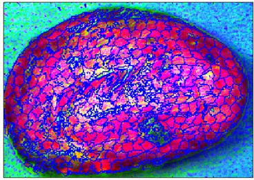
where H c is the sum of the RGB distance and the xy plane distance normalized by the grid interval S; and r j , g j , and b j denote the color of the j- th superpixel cluster center, while j' indexes each pixel, j' = [1, MN]. The value of m controls the compactness of a superpixel, which can be in the [1,20] range. Usually, it is chosen as =10 [39]. In this paper, we used N spx =500.Figure 6 is an RGB image segmented into superpixels with the SLIC algorithm and displayed with a false-color composite.
Source: Authors’ own work.
Figure 6 A cocoa bean RGB image segmented into 500 superpixels with the SLIC algorithm
Finally, the spatial information of the superpixel map is matched with the hyperspectral information of the data cube
to calculate the average spectral signature of each superpixel and build an array with these spectral signatures, i.e., a matrix of size L×N
spx
, as explained below.
Let
∈ R
L × MN
be the unfolded matrix of the hyperspectral image (
) reorganized as
= [
(1),…,
(MN)], where
(k)
∈ R
L
represents the spectral signature of the k-th pixel.
Mathematically, the matrix with the average spectral signatures Y∈R L×Nspx is created as (9):

where H ∈R MN×Nspx is an average sorting matrix, in which the different values of zero for each column (ℓ) have a weight 1⁄( N s ℓ ), such that N s ℓ is the number of pixels grouped in a superpixel. Then, the matrix Y= [y 1,…,y Nspx ] of spectral signatures will be classified as explained in the next subsection.
2.5 Supervised Classification
The last step in the proposed framework is to classify the spectral signatures of each superpixel in Y using the Support Vector Machine (SVM) algorithm.
For this purpose, we denote the information of n spectral signatures used in the training step as Θ= {y1,…,yn }, and their respective class labels as Ω={ω 1,ω 2,ω 3}, where ω 1, ω 2, ω 3 ∈ R n/3 represent the slight, correctly, and high fermentation levels, respectively.
2.5.1 Algorithm
The SVM algorithm was initially proposed for binary classification in order to determine a hyperplane (y T k M+b) that optimally separates the samples of one class from those of another [42] , [43]. However, since this study considers three categories, multiple-class SVM should be employed [42]. However, since this study considers three categories, multiple-class SVM should be employed [43]. Specifically, said method seeks to determine d hyperplanes (in our case d = 3), solving the following optimization problem for the training stage (10):

where M
m
is the m-th weight vector; n, the number of training samples; ωi ∈ {1, ... ,d}, the labels of the i-th super-pixel;
 the set of slack variables that consider the nonseparability between sets belonging to different classes; λ, a regularization parameter that controls the influence of the misclassified samples; i=1,...,n; and t∈1,...,d. The mapping function φ projects the training data into a suitable feature space to allow for nonlinear decision surfaces, and δ
i,j
is the Kronecker delta function with value 1 for i=j and 0 otherwise. Finally, with trained weight vectors M
m
, the resulting decision function for any superpixel y
i
is given by (11):
the set of slack variables that consider the nonseparability between sets belonging to different classes; λ, a regularization parameter that controls the influence of the misclassified samples; i=1,...,n; and t∈1,...,d. The mapping function φ projects the training data into a suitable feature space to allow for nonlinear decision surfaces, and δ
i,j
is the Kronecker delta function with value 1 for i=j and 0 otherwise. Finally, with trained weight vectors M
m
, the resulting decision function for any superpixel y
i
is given by (11):

Note that the result obtained in (11) is the classification of one superpixel. Therefore, to assign a label to the whole bean, the predominant label is calculated as (12)

3. DATA ANALYSIS AND RESULTS
This section presents an analysis of the classification of cocoa beans in terms of their level of fermentation using the proposed method. The SVM classifier uses a Gaussian kernel and cross-validation for hyperparameter tuning, which was implemented using a Matlab toolbox.
First, the classification focuses on finding a label for each bean based on the calculation of the predominant label. Second, bean uniformity is analyzed assuming each superpixel as a sample. Finally, the influence of the number of training samples on classification accuracy is calculated.
3.1 Bean Classification Based on Predominant Label
In this subsection, we evaluate the classification proposed in (12). The objective is to label each bean with its predominant fermentation category. Table 2 lists some parameters of this classification.

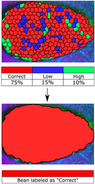
In total, we classified 90 cocoa beans, each one spatially divided into 500 regions (superpixels); that is, we classified a total of 45,000 superpixels. Let us remember that each superpixel has an associated spectral signature consisting of 301 reflectance values measured between 350 and 950 nm in steps of 2 nm. For this classification, we used 15 % of the samples to train the SVM classifier. Figure 7 shows the result of classifying one of the 90 cocoa beans using the proposed method. The framework assigns a label to the spectral signature of each superpixel and, subsequently, assigns the predominant label to each bean.
Source: Authors’ own work.
Figure 7 Visual results of the classification by superpixels (top) and predominant label (bottom)
As mentioned in Subsection 2.1, we also had the reference label of each bean, which was carefully assigned by a professional technical team. Therefore, after assigning a label to each bean, this method evaluated the precision of the classification proposed in this paper by comparing the results with the reference labels.
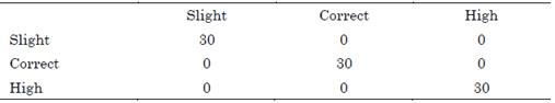
The confusion matrix in Table 3 details the number of beans correctly and incorrectly labeled with the proposed method. Each column in the matrix represents the number of predictions of each class, while each row represents the ground truth.
Table 3 Confusion matrix of all the beans classified based on the predominant label (Equation 12)
Source: Authors’ own work.
From the results in the confusion matrix, we calculated the values of recall, precision, truth overall, and overall classification per class as in [44]. These results are shown in Table 4.

Note that all Slightly, Correctly, and Highly fermented cocoa beans were correctly labeled by the classifier (Table 3). In addition, the metrics in Table 4 show the high performance of the proposed classification approach. The overall precision of assigning the predominant label to 90 cocoa beans was 100 %.
3.2 Bean Uniformity Analysis
Entities that regulate the international marketing of cocoa beans, such as The Federation of Cocoa Commerce London (FCC), require the quality of the seeds in each ton to be acceptably uniform. The objective is to guarantee the homogeneity of the products derived from cocoa.
An approach such as the one proposed here can be used to analyze the uniformity of cocoa loads. It was shown that the 90 beans used in this study were correctly classified, 30 into each one of the fermentation categories. However, note that the initial labeling of the bean (bottom, Figure 7) disregards the fact that some superpixels can be classified into other fermentation levels different from the predominant one (top, Figure 7). Therefore, classifying each superpixel in a grain separately, we can analyze how uniform each bean is.
In this subsection, we discuss a more detailed classification in which bean fermentation uniformity is calculated. This type of analysis has not yet been used commercially in the cocoa industry. Furthermore, it is rarely used in general food quality control, where uniformity is assessed at the collective level (batch uniformity).
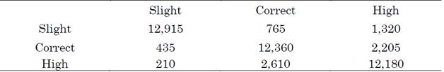
Table 5 shows the result of classifying the average spectral signature of each one of the 45,000 superpixels. We used the general bean category as the reference label for each superpixel in the confusion matrix. Note that, compared to Table 3, the matrix in Table 5 is not diagonal. It is understood that the matrix is not diagonal because there may be regions (superpixels) with different degrees of fermentation despite being on the same grain.
Table 5 Confusion matrix of all the classified spectral superpixels (Eq. 11)
Source: Authors’ own work.
Table 6 shows the percentage of superpixel classification in each class. The rows represent the actual labels (full-grain categories); therefore, the sum of the values in each row is equal to 100 %. In turn, the columns show the tags assigned by the classifier to the superpixels. The last row, Total, shows the percentage of superpixels labeled by the model in each fermentation level. Note that, although there are 30 beans in each category, regions of correct and high fermentation predominate, with 34.96 % and 34.89 % of the areas, respectively.

Furthermore, Table 6 shows that, in highly fermented beans, there is a considerable amount of material that is well fermented (17.4 %), and vice versa (14.7 %). In comparison, only small portions of the beans with high and correct fermentation have slight fermentation (1.4 % and 2.9 %, respectively). Regarding slightly fermented beans, there are small burned regions (high, 8.8 %) and a minority of well-fermented areas (5.1 %).
This analysis could contribute to the implementation of fermentation techniques that produce a more homogeneous drying.
3.3 Number of Training Samples and Classification Accuracy
In this subsection, we vary the number of spectral signatures per category used in the SVM classifier training in order to analyze its influence on the precision of the classification and determine how many spectral signatures are necessary to obtain acceptable results.
The training was programmed to randomly select a certain percentage of spectral samples, the same number of signatures from each category. The system was trained, and the beans were classified using the predominant label method. Specifically, the percentage of training samples was varied between 1 % and 20 % of the total signatures (45,000), as seen on the x-axis in Figure 8. A 10 % of each resulting training set was used as validation to tune the model.
Figure 8 shows the average accuracy of the test set over ten experiments. Evidently, as the number of training samples increases, the classifier improves its precision.
Note that the class most easily recognized by the classifier is Slight fermentation, followed by Correct and High, with any proportion of training samples.
Specifically, using only 2.5 % of the training samples (which is equivalent to 1,125 spectral signatures), the system correctly labeled 90 % of the cocoa beans as Slight fermentation, i.e., 27 of the 30 beans in this class. Likewise, with the same training percentage, the classifier accurately detected 76.6 % of the beans with Correct fermentation (23 beans), and 63.3 % of those with High fermentation (19 beans).
Furthermore, in Figure 8, when the percentage of training samples exceeds 12.5 %, the overall accuracy of the classification is quite acceptable. In fact, let us remember that the results in Subsections 3.1. and 3.2. were obtained from classifications performed with 15 % of the training samples.

4. CONCLUSIONS
In this paper, we developed a non-invasive framework for classifying dry cocoa beans into three fermentation categories using spectral imaging and no chemical methods. The evaluation of the performance of the proposed framework showed its high accuracy in the classification of cocoa beans when 15 % or more of the samples in each category were used for training. Subsequently, the results were compared with the labels assigned to each bean by the Colombia National Federation of Cocoa Growers. The results of this study demonstrate that the use of spectral information is feasible for the noninvasive quality control of cocoa beans.
Furthermore, using the proposed classification framework, it is possible to establish the percentage of each bean that belongs to a fermentation category different from the label of the whole bean. Future studies should examine other classification methods and frameworks in order to compare their computational complexity and accuracy with those of the SVM approach.
The implementation of an analysis with this level of detail in the productive sector can help to investigate fermentation techniques that yield more uniform results. In the business sector, it can allow organizations to improve their pricing methods and have a more demanding selection of raw material for premium-quality products derived from cocoa.

