


 English (pdf)
 Article in xml format
 Article references
 Send this article by e-mail
 Cited by SciELO
  Cited by Google
  Similars in
SciELO
Similars in
SciELO  Similars in Google
 Permalink
Introduction
Geothermal energy refers to the heat produced inside the Earth. This energy is transported to the surface through water or steam (DiPippo, 2015), and is considered one of the cleanest and most renewable energy sources on the planet (Dickson & Fanelli, 2003). Geothermal fluids are used to produce electricity and have several applications, including space heating, geotourism, and health, among others (Lund & Boyd, 2015).
The geothermal area of Paipa is located in the eastern cordillera of Colombia, south of the Paipa town, with a surface area of130 km2 (Figure 1). In this area, geothermal fluids rise to the surface in two specific areas; these fluids are currently only used in baths and thermal pools. Different investigations have been carried out to evaluate the geothermal potential of Paipa (Alfaro Valero C., 2002; Vásquez L., 2002; Velandia F., 2003; Cepeda & Pardo, 2004; Alfaro Valero & Espinoza, 2004; Alfaro Valero C. 2005; Alfaro Valero C., 2005b; Ortiz & Alfaro, 2010; Franco J., 2012; Vásquez L., 2012; Rodríguez & Vallejo, 2013; Llanos et al., 2015; Moyano I., 2015; Rueda J., 2016). Although several studies have assessed the geothermal system of Paipa, no research has included satellite information with thermal infrared.
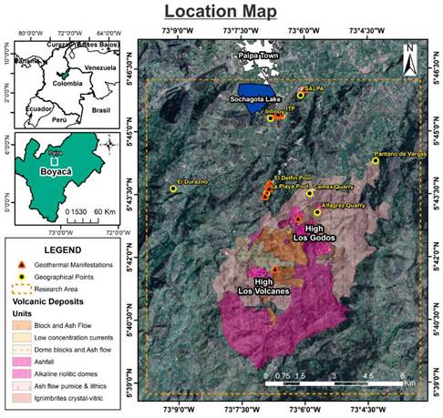
Figure 1 Location of the study area in Paipa-Boyacá, Colombia (the orange dashed rectangle marks research area). The red edge triangles represent main geothermal manifestations, and yellow edge circles represent well know geographic reference points. Finally, color polygons represent the volcanic deposits at zone.
Thermal remote sensing has been used effectively in the exploration of geothermal resources, resulting in saving resources such as time and money, it is shown by several geothermal explorations of active volcanoes and other geothermal areas (Zhou, 1998; Ayenew, 2001; Qin et al., 2011; Norini et al., 2015; Chan et al., 2018; Darge et al., 2019). Some of these investigations have been carried out in well known geothermal areas, allowing the identification of new specific areas of geothermal interest (Coolbaugh, 2003, Gutiérrez et al., 2012). Multispectral satellites, such as Landsat 7 ETM+ and Landsat 8 OLI/TIRS, have thermal bands that are used to determine thermal anomalies in volcanic areas and geothermal areas (Mia et al., 2014, Chan & Chang, 2018, Cesarian et al., 2018; Sekertekin & Arslan, 2019). The use of thermal satellite images has some limitations; not all scenes are of a high quality due to cloudiness and spatial resolution, and due to difficult access in some areas, validation of satellite data with field data is challenging.
Landsat 7 ETM+ has a thermal band with a spatial resolution of 60 m and a spectral range between 10.4 and 12.5 µm. A single-channel algorithm was applied to this band to determine surface temperature anomalies (Jiménez- Muñoz et al., 2009). Similarly, Landsat 8 OLI/TIRS has two thermal bands with a spatial resolution of 100 m and a spectral range between 10.6 to 11.19 µm (band 10) and 11.5 to 12.51 µm (band 11). A two-channel algorithm (Split Window) was applied to these two bands (Du et al., 2015).
The exploration of Paipa geothermal area is being carried out for the first time by thermal satellite images. The approach used here aims to demonstrate the effectiveness of the thermal infrared satellite to determine geothermal anomalies, supported by field measurements that allow the validation of satellite data. The main objective of this research is to highlight exploratory prospects in order to the Paipa community to take advantage of new hydrothermal fluids and attain economic growth in the region.
Geological and Geothermal Framework
Paipa geothermal system is located in the eastern cordillera basin whose geological units are mainly sedimentary, with ages ranging from -130 m.y., to the present (Figure 2). The formations of Cretaceous period correspond to Tibasosa-K1t (limestone and mudstone), Une-K1u (quartz sandstones), Churuvita group-K2ch (mudstone and sandstone), Conejo-K2c (mudstone, siltstone, and limestones), Plaeners-K2pl (siltstone and chert), Los Pinos-K2p (mudstone and siltstone), Labor-Tierna-K2lt (quartz sandstones) and Guaduas-K2E1g (mudstone, sandstones and coal). From the Paleogene period, Bogotá formation-E1-2b (quartz sandstones). From the Neogene period the Tilatá formation-N1t (sandstones and mudstones), and pyroclastic volcanic deposits and intrusive domes. Also, from the Quaternary, there are colluvial (Qc), and fluvial-lacustrine (Qal) deposits located in the flat parts of the zone (conglomerates and sandstones) (Velandia, 2003). As for the volcanic deposits, these are located seven kilometers south of Paipa town (Figure 2) and are classified mainly as ash flows, ash falls, and dome blocks; the body domes composition is rhyolitic (Cepeda & Pardo, 2004). Outcropping on the surface, there are 18 geothermal manifestations, mainly hot springs and a steam vent (Figure 2) (Alfaro et al., 2017). Previous reports such as that of the Latin American Energy Organization (OLADE, ICEL, CONTECOL & Colombian Geotermia, 1982) and the Japan Consulting Institute (1983), conceptualized that this area has a geothermal interest classified from medium to high, with a possible geothermal reservoir suitable for its exploitation. Rodríguez (1998) determined that the volume of thermal water available in the area is approximately 480,000 m3. The Colombian Geological Service (CGS) proposes a source of magmatic heat, associated with the heat remaining from igneous intrusions and/or heat from radiogenic minerals, which heats the waters of the system (Alfaro Valero et al., 2017). Also, the CGS proposes the existence of two hydrothermal systems, one primary and the other secondary, for its possible temperatures in depth; the primary system would be generated by infiltration of surface water at a depth between 4 and 5 km, which would circulate from the SE of the area to the NW, reaching temperatures higher than 230°C. The secondary hydrothermal system located NW of the area, where surface water would infiltrate to a depth of 1.5 km, reaching a temperature around 75°C, restricted laterally by the Canocas and Hornitos faults, superficially this system does not show hot springs.

Materials and methods
Satellite Data
Satellite images are primary information sources in this investigation. These images include scenes from Landsat 7, Landsat 8, MODIS/Terra, ALOS-PALSAR and Pléiades. Land surface temperature anomalies are determined using spectral bands of red (30m / pixel), near infrared (30m/ pixel) and thermal infrared (60m-100m/pixel) of Landsat images. We also used spectral radiance images (MOD021KM) and images of water vapor content of the product MOD05L2 (1000m/pixel) of MODIS/ Terra, which is used to correct the thermal emissivity of the surface atmospherically. The digital elevation model-DEM (12.5m/pixel) used was obtained from the ALOS-PALSAR product, and the Pléiades image of the high-resolution visible spectrum (RGB) (0.5m/pixel) were used in conjunction with the DEM to create anaglyphs.
The images cover path 7 and row 56 of Landsat images. In order to multi temporarily analyze the thermal anomalies, five Landsat diurnal images were used. These were acquired on the dates 2000-12-13, 2001-01-30, 2002-01-17, 2002-03-06, 2003-01-04 for Landsat 7 and 2016-02-01 for Landsat 8. These images were selected because they presented 0% cloudiness for the research area and are of excellent quality.
Field data
Like satellite images, field data is primary information. We acquired fifty field stations of solar radiation, soil, air, and surface temperatures, relative humidity, and atmospheric pressure. A radiometric station RS (powered by solar energy) and a FLIR CAT-S60 thermal camera were used. The RS (Figure 3) is composed of a data logger, a solar panel, a radiometer, an infrared radiometer, a thermistor, and a multiparameter environmental sensor. Table 1 provides details of the RS sensors.

Table 1 Instruments used in the field data collection
| Variable | Units | Sensor | Brand / Model |
|---|---|---|---|
| Soil Temperature | °C | Thermistor | Apogee/ ST100 |
| Surficial Temperature | °C | Non-contact Infrared thermometer | Apogee/ SI-4H1 |
| Object surficial Temperature | °C | Thermal camera | CAT FLIR / S60 |
| Air Temperature | °C | VP-4 | Decagon / PASSRHT |
| Vapor pressure | kPa | ||
| Relative Humidity | % | ||
| Atmospheric Pressure | kPa | ||
| Incident and reflected solar radiation | W/m2 | Net Radiometer | Apogee/ SN500 |
| Net Radiation | W/m2 |
Solar radiation, air, and surface temperature data were used to correct and validate the temperature values of the satellite images. The soil temperature data was used to create a map of soil temperature anomalies in the area.
Methodology
This study was carried out in five stages (Figure 4). First, the reference information was established; second, the satellite images were processed digitally; third, index maps were defined; fourth, a spatial model was applied to the four index maps, and finally, the hydrothermal prospects were defined.

Digital image processing
This stage consists of three steps. First, the Landsat bands were radiometrically calibrated and atmospherically corrected. Second, the red and infrared near bands were used to calculate the thermal emissivity of the surface. Finally, the algorithms of a single thermal band (Jiménez-Muñoz & Sobrino, 2003) and two Split-Window thermal bands (Du et al., 2015) were used to determine the thermal anomalies of the surface. The following sections provide a detailed description of each of these procedures.
Land Surface Temperature retrieval
The first step to obtaining surface temperature images is the conversion of digital numbers (DN), in spectral radiance values (Lλ to the top of the TOA atmosphere (Chander et al., 2009). For Landsat 7 and Landsat 8 images equations (1) USGS (2018) and (2) USGS (2016) were used.

Where, G rescale , B rescale , M L and A L , are specific rescaling factors for each band; they are found in the metadata of each of the images. Qc a l is the raw value of each pixel in the images, for the case of Landsat 7, those values are between 0 and 255, and for the Landsat 8 images values are between 0 and 65,535.
Atmospheric Correction
Atmospheric effects correct the bands in the visible and near-infrared spectrum. This correction is applied due to absorption and dispersion processes, as a result of the existence of water vapor, gases (Ozone, Oxygen, Carbon Dioxide, Nitrogen Oxide, etcetera.) and molecules in the atmosphere, which affect the amount of radiation received by the sensor. These atmospheric effects are removed in order to obtain an image of spectral reflectance whose values reflect real physical magnitudes of the surface. To obtain atmospherically corrected images, the atmospheric correction module Fast Line-of-Sight Atmospheric Analysis of Spectral Hypercubes (FLAASH) was used. In general, FLAASH is an atmospheric correction method based on the MODTRAN 4.0 Radiative Transfer code, which allows the removal of the effects of dispersion and absorption in the Multispectral and Hyperspectral images, which was developed by the Laboratory of the US Air Force. (Kayadibi, 2011).
Thermal emissivity calculation
Once the red and near-infrared bands were corrected atmospherically (Example: bands 3 and 4 for Landsat 7), the values of surface emissivity were determined. The approach used here is the one proposed by Sobrino et al., (2004), it is based on the determination of the emissivity for each pixel, based on the proportion of vegetation Pv, obtained from the values of the Normal Differential Vegetation Index (NDVI), equation (3).

The method is called NDVI thresholds (NDVITH), which considers three different surface classes, dependent on the NDVI values: a) Bare soil (NDVI <0.2), b) mixed surface (0.2>NDVI<0.5), and c) Surface fully covered with vegetation (NDVI> 0.5).
a) Bare soil (NDVI <0.2): The emissivity value for Landsat 7 images is established as constant ε = 0.97. In the case of Landsat 8 images, the emissivity was determined from the reflectance of the red band ρred, for each of the thermal bands, ε10=0.973- 0.047 ρ red and ε11 = 0.984 - 0.026 ρ red (Yu et al., 2014).
b) Mixed surface (0.2 > NDVI < 0.5): The pixels are considered as a mixture between vegetation and bare soil. The emissivity is obtained as a function of the proportion of vegetation, as follows, ε = ε v P v + ε s (1 - P v ) + de, where, ev is the emissivity of the vegetation, ε s is the soil emissivity, and de is a term which includes the effect of geometric distribution of natural surfaces and internal reflections (Sobrino et al., 2004). The proportion of vegetation is calculated
from the following equation,
 where, NDVI
min
= 0.2 and NDVl
max
= 0.5. de is calculated in the following way d ε = (l - ε
s
)(l- P
v
)*F * ε
v
, where F is a form factor, with a mean value of 0.55, which considers different kinds of geometric distribution.
where, NDVI
min
= 0.2 and NDVl
max
= 0.5. de is calculated in the following way d ε = (l - ε
s
)(l- P
v
)*F * ε
v
, where F is a form factor, with a mean value of 0.55, which considers different kinds of geometric distribution.
For the case of the Landsat 8 thermal bands, the average emissivity values of the soil and vegetation of each one were taken into account: εs10= 0.9668, ε s11= 0.9747, εv10= 0.9863, εv10= 0.9896 (Yu et al., 2014).
c) Surface fully covered with vegetation (NDVI> 0.5): It was assumed for both Landsat 7 and Landsat 8 images, a constant value e = 0.99.
Calculation of Surface Kinetic Temperature
Two algorithms were chosen to determine the kinetic surface temperature of Paipa's geothermal area. For the Landsat 7 ETM + thermal band, the one-channel algorithm proposed by Jiménez-Muñoz & Sobrino (2003) was used, and for the Landsat 8 TIRS thermal bands, the Split-Window algorithm, proposed by Du et al., (2015) was used. These two algotthmsare b+sedon the radiative transfer equation (RTE), equation (4). T his equation expresses the law of Planck, defining that the spectral radiance B(λ,T) of a black body is a function of the wavelength A(m) of the electromagnetic energy and the absolute temperature of the body T(K).

Where c1 and c2 are constants of Planck, with values of 1.19104 * 108 W.µm4.m-2.sr-1 and 14387.7 um.K, respectively.
Single Channel Algorithm (SC)
Jiménez-Muñoz & Sobrino (2003) and Jiménez-Muñoz et al., (2009) proposed an algorithm to determine the surface temperature LST, from a single channel, equation (5), based on the concept of Atmospheric Functions (FAts), which depend on the atmospheric transmissivity and the descending and ascending atmospheric radiations.

Where e is the emissivity of the surface; y and S are two parameters dependent on the Planck functions, expressed in the following way,
 and
and
 Where Tsen is the temperature of brightness in the sensor (equation 6); by is a constant, with a value of 1277 K for Landsat 7 and Lsen is the spectral radiance in the sensor. Finally, φ1, φ2, φ3 are atmospheric functions, φ1= 0.14714ω2 - 0.15583 ω +1.1234; φ2 = -1.1836ω
2 -037607 ω 052894; − φ3= 0.04554ω2 + 1.8719ω -0.39071, where ω is the water vapor content (WVC) in the atmosphere in g/ cm2. The product MOD05L2 of the MODIS sensor, offers continuous values of to at a spatial resolution of 1 km2, being appropriate due to the small spatial variation of to in the atmosphere (Ren et al., 2015).
Where Tsen is the temperature of brightness in the sensor (equation 6); by is a constant, with a value of 1277 K for Landsat 7 and Lsen is the spectral radiance in the sensor. Finally, φ1, φ2, φ3 are atmospheric functions, φ1= 0.14714ω2 - 0.15583 ω +1.1234; φ2 = -1.1836ω
2 -037607 ω 052894; − φ3= 0.04554ω2 + 1.8719ω -0.39071, where ω is the water vapor content (WVC) in the atmosphere in g/ cm2. The product MOD05L2 of the MODIS sensor, offers continuous values of to at a spatial resolution of 1 km2, being appropriate due to the small spatial variation of to in the atmosphere (Ren et al., 2015).

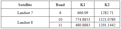
Where, K1 [W.m-2.sr-1.µm-1] and K2 [K] are calibration constants (Table 2); L λ is the spectral radiance in the sensor [W/(m2.sr.µm)] and ln is the natural logarithm.
Table 2 Calibrations constants used to convert spectral radiance in brightness temperature, for Landsat 7 ETM+ and Landsat 8 TIRS.
Before being able to use the MODIS images, a process of georeferencing of the MOD021KM products was carried out, starting from the Landsat images. Once the MOD021KM images were georeferenced, a co-registration process was performed with their respective MOD05_L2 images, obtaining correctly geo-positioned WVC images. Once the WVC images were correctly geo-positioned, their values were validated using the values of relative humidity and air temperature, collected in the field, by applying equation 7, where T0 is the surface air temperature, RH is the relative humidity of the air and WVC is given in g/cm2.

The WVC values obtained from the field data vary from 0.52 g/cm2 to 1.46 g/cm2, which are very similar to the average values of WVC obtained by the MODIS sensor in each of the dates of the Landsat images (Table 3). This similarity allowed the validation of the WVC satellite values.
Table 3 Water vapor content statistics of the MOD05L2 images, for each of the dates used in Landsat.
| Statistics | MOD05 20001213 | MOD05 20010130 | MOD05 20020117 | MOD05 20020306 | MOD05 20030104 |
|---|---|---|---|---|---|
| Min | 0.577282 | 0.486306 | 0.369391 | 0.706861 | 0.955387 |
| Max | 1.54891 | 0.93637 | 1.032812 | 1.71515 | 2.12305 |
| Mean | 1.147071 | 0.651245 | 0.749141 | 1.145315 | 1.33665 |
Split Window Algorithm (SW)
Du et al., (2015) proposed a practical algorithm, which takes advantage of the two thermal bands of the TIRS sensor, onboard the Landsat 8 satellite. The algorithm obtains the surface temperature from a linear relationship, with the combination of the brightness temperatures of the two thermal bands, with clear sky conditions. Like the algorithm of Jiménez-Muñoz & Sobrino (2003), the SW is based on the theory of radiative transfer, so it is necessary to have atmospheric information at the time of image acquisition. To solve this, the algorithm of equation (8) depends on eight coefficients, which vary depending on the WVC, at the moment of image acquisition. The coefficients were calculated from a modified SW method of covariance-variance relation, obtaining five different ranges of WVC, [0.0 - 2.5], [2.0 - 3.5], [3.0 - 4.5], [4.0 - 5.5], and [5.0 - 6.3] g/cm2.

Where Ti and Tj are the brightness temperatures of bands 10 and 11, respectively; ε is the average emissivity of the thermal bands
 is the difference of the emissivity ∆ε = εi.- εj., and b0, b1, ...b7 are the coefficients determined for each WVC range. The coefficients used correspond to the values defined for a range of WVC between 0.0 and 2.5 g/cm2, determined thanks to the record of the MODIS images and the field values, whose average value is 1.3 g/cm2.
Obtaining Structural Lineaments
The first step to obtain the structural lineaments, was to combine the ALOS-PALSAR (DEM) scenes in a single image; for this, the mosaic tool of ERDAS Imagine 2018® was used. Subsequently, shadow models were obtained; these models were combined with the DEM and the Pléiades images of the visible spectrum, thus obtaining three-dimensional images (anaglyphs). Once the anaglyphs were obtained, the structural analysis of the geothermal area of Paipa was carried out. The deformation structures were interpreted visually, using the 3D views of the anaglyphs. The lineaments were mapped using a geographic information system (GIS). Moreover, the identified structures were verified with the existing geological information (Velandia, 2003) and the fieldwork carried out in this study.
Iso-resistivity map
Based on the reference information, the iso-resistivities map published by the CGS (Franco, 2016 in Alfaro Valero et al., 2017) was used. This iso-resistivity surface information was measured at an elevation of 2,500 m.a.s.l., and the anomalies of low resistivity indicate the location of geothermal fluids in the area.
Soil Temperature Map
A soil temperature map of the Paipa geothermal system was made. One hundred ninety-seven temperature probes were used, recorded at depths greater than one meter. The Geostatistical wizard tool of ArcMap© was used by applying an interpolation method of kriging. The one hundred ninety-seven soundings are constituted by 147 soundings taken by the CGS (Rodríguez & Vallejo, 2013) and 50 new temperature data acquired in the field throughout this study.
Spatial Model
The maps obtained from satellite surface temperature (Sst), structural lineaments (Sl), iso-resistivity surface (Is), and soil temperature (St) were integrated in an unweighted way into a spatial model. Three index values were defined to each of these maps, corresponding to the areas of higher temperature (SST and St), areas of influence of the structural lineaments (Sg) and areas of lower resistivity (Is). The model was based on obtaining a spatial relationship between the four index maps. To achieve this, the Union spatial function, offered by ArcMap©, was used. The result obtained called Integrated Index Map (Ii), corresponds to new polygons, containing in their attributes the values of the indexes that were superimposed (Figure 5). Finally, the index values in each polygon were summed and divided into the total number of indexes (Equation 8).

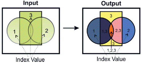
Figure 5 Illustrative diagram of the result obtained from the Union process. The input data is three layers, each with a defined attribute value (1, 2 and 3); the result presents the same figure, but now there are seven different polygons, and each contains a different number of attributes; note the orange polygon now contains the attribute values 1, 2, and 3.
Index Maps
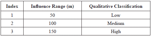
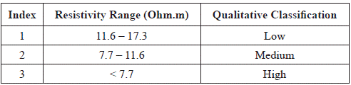
The index maps correspond to geophysical and geological indicators, which have a spatial relationship with the occurrence of hydrothermal fluids on the surface; each index was classified into three qualitative ranges depending on their temperature, resistivity and lateral area of influence of the lineaments. The defined index values are 1, 2, and 3, classified qualitatively as, low, medium, and high probability, respectively.
a) Surface temperature index map
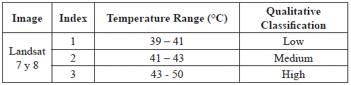
Two of the thermal satellite images were integrated. The images used correspond to a Landsat 7 ETM+ of March 6th, 2002 and a Landsat 8 TIRS of February 1st, 2016. These images were selected for the dominant surface coverage on those dates. The ground covers correspond to surfaces mainly of half-bare soil, and this is ideal since the temperature values can be affected by the evapotranspiration processes of the vegetation. Thus, the resulting temperature anomalies of the images are similar in shape and magnitude. Table 4 presents the index values defined for the three highest temperature ranges of satellite thermal images.
Table 4 Satellite temperature indices. Three ranges of maximum temperature were defined and classified qualitatively.
The temperature anomalies of the two Landsat images were classified according to Table 4, later, they were converted into a vector format, and the ArcMap© union process was applied. The result obtained corresponds to the integrated temperature anomalies of the two satellite images (Figure 12-a).
b) Lineaments Index Map
Based on the mapped lineaments, three influence areas (buffer) were established around them. These three areas correspond to the three established rates, low, medium, and high probability of allowing the circulation of hydrothermal fluids (Table 5). The index map of structural lineaments is presented in Figure 12-b.
Table 5 Indices of lineaments. Three influence distances were defined with their respective qualitative classification.
c) Iso-resistivity index map
From the iso-resistivities surface (figure 10), the index values of this map were defined. The values of resistivity found in the zone vary between 0 and 2,251 Ω2.m, and according to the geothermal conditions of Paipa, it was interpreted that the low values of resistivity between 0 and 17.3 Ω.m, are the result of hot saline fluids (Ussher et al., 2000). These low values of resistivity were taken and classified in the three index ranges (Table 6), defining the iso-resistivity index map (Figure 12-c).
Table 6 Indices defined for three minimum ranges of subsoil resistivity, with their respective qualitative classification.
d) Soil temperature index map
A frequency analysis of the soil temperature data was carried out, concluding that the majority of the data set corresponds to values without geothermal influence, that is, the values of temperature between 15 °C and 19 °C. On the other hand, it was established that the temperature data between 19.1 °C and 37 °C correspond to values with geothermal influence (Figure 6). From this last temperature range, the index values were established (table 7), and the soil temperature index map was obtained (Figure 12-d).


Prospects
The prospects of the Paipa geothermal area were obtained by making a spatial superposition of the four index maps. The objective was to identify the areas where the highest index values were superimposed (index value 3), that means, high satellite temperature, high soil temperature, low electrical resistivity and proximity to the fault zone.
Results and discussion
Land Surface Temperature Anomalies
The results of the Landsat bands processing are presented in figure 7. The application of the algorithms proposed by Jiménez-Muñoz & Sobrino (2003) and Du et al., (2015) in the thermal bands of Landsat 7 ETM+ and Landsat 8 TIRS, allowed to correct in these, the effect of the emissivity of the surfaces and the processes of dispersion and absorption generated by atmospheric conditions, mainly due to the effect of the water vapor content in the atmosphere. The correction of WVC in the atmosphere was carried out satisfactorily with the MOD05L2 products, for the case of the "Single Channel" algorithm and the case of the "Split Window" algorithm with the chosen range of water vapor content between 0.0 and 2.5 g/cm2. This was due to the atmospheric data of temperature and relative humidity of the air, acquired in the field, which allowed it to validate the research areas with an average WVC value of 1.3 g/ cm2, validating the values of WVC recorded by the MODIS sensor and the chosen range for the "Split window" algorithm.
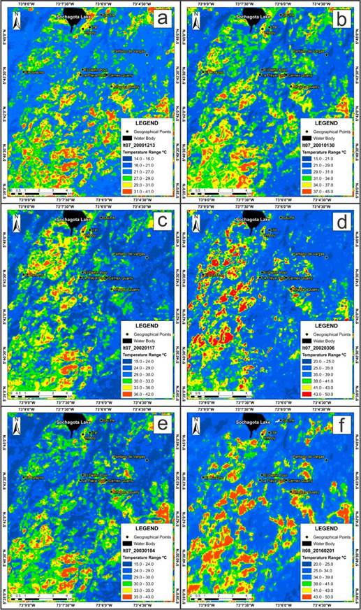
Figure 7 Anomalies of land Surface temperature from Landsat 7 ETM+ on December 13, 2000; January 30, 2001; January 17, 2002; March 06, 2002; January 04, 2003; and Landsat 8 TIRS on February 01, 2016.
Another relevant aspect of the application of the algorithms is obtaining surface temperature anomalies with higher temperature magnitudes, and the reduction in the size of the anomalies in comparison with the temperature anomalies obtained without the atmospheric and emissivity corrections (Temperature of brightness). As an example, Figures 8a and 8b are compared, and it is possible to observe the differences in the size of the temperature anomalies, being of much larger extension for the temperature anomalies of brightness, while the temperature anomalies where the corrections are applied have a smaller size and their magnitude (temperature) is higher. Regarding the variation of the temperature magnitudes, there was a generalized increase of around +8°C, for the hottest anomalies, while for the colder temperature anomalies there was an increase of around 3.5°C.
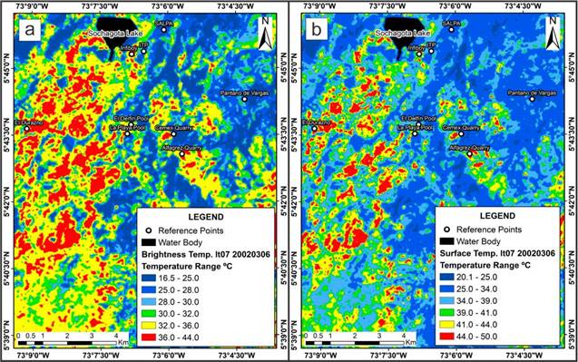
Figure 8 Comparative images between the satellite thermal anomaly sizes, from the Landsat 7 EMT+ scene, of March 6, 2002. a) Brightness temperature image. b) Surface temperature image.
The satellite thermal anomalies reflect an excess of heat coming from the interior of the earth. Thus, in areas of geothermal activity, the images of surface temperature that are obtained have two sources of energy, one coming from solar heating and another coming from the interior of the earth. The equation of the surface energy balance (equation 9) allows us to comprehend how it is possible to identify zones with geothermal activity.

Where Qn is the net solar radiation received by the surface; H is the sensible heat flow between the ground floor interface; λE is the latent heat flux in the transition phase of water between the surface and the atmosphere; G is the heat flow of the soil. Locally, it is assumed that H and λE have little influence on surface thermal anomalies so that the net radiation and the heat flow from the soil are those that would generate the signature of heat registered by the sensor.
Structural Lineaments Map
Figure 9 presents the map of structural lineaments obtained from the 3D interpretation. The result shows the existence of a dense network of fractures which would affect the geothermal area of Paipa. The lineaments validated in the field and reference information corresponds to the Hornito, Canocas, El Batán, El Bizcocho, Cerro Plateado, and Las Peñas faults.

Iso-resistivity Map
Figure 10 shows the iso-resistivities surface of the Paipa geothermal area. Resistivities under 17.3 Ωm were interpreted as a result of a geothermal source. Six specific zones of high conductivity (<2.3 Ωm) were identified in the study area. The anomaly 1 in the north of the area, is not taken into account because this anomaly is generated by a deposit of salt in that area. The other anomalies are interpreted as shallow accumulations of geothermal fluids.

Soil Temperature Map
Figure 11 shows the soil temperature map, with data acquired at one-meter depth. The presence of six anomalous zones is clearly identified, with two principal anomalies, one located to the east of Sochagota lake (anomaly 1) and the second to the south, in the sector of the El Delfín and La Playa pools (anomaly 4), each corresponding spatially to the zones where the geothermal manifestations of the zone are presented. In general, there is a spatial correlation between resistivity anomalies and soil temperature anomalies, mainly between anomalies number 2 and number 1 (Figure 10 and 11), anomalies 3-4-5 with anomaly 4 (Figure 10 and 11), and the number 6 of the two anomalies (Figure 10 and 11).

Spatial Model - Index maps
The implemented spatial model took into account indicators with a spatial relationship with the presence of hydrothermal fluids (Figure 12). Lineaments act as migration paths or may restrict the lateral distribution of hot fluids. The resistivity anomalies reflect the possible zones of accumulation of geothermal fluids because these fluids have physical and chemical properties characteristic of temperature and salinity, which produce very high conductivities. Soil temperature anomalies at shallow depths are the direct manifestations of heat transfer from the subsoil to the surface, with convection being its transfer mechanism. Finally, the thermal anomalies obtained from the satellite images are the continuous representation of the surface temperatures mainly product of the interaction between the solar radiation and the heat coming from the interior of the earth, which allows identifying anomalously hot zones through the surface. These variables integrated from a geographic information system, in an unweighted way, facilitated the spatial correlation between each of them and allowed for the application of a simple algorithm with which it was possible to generate point zones, which are assumed as the areas of most significant probability to find new hydrothermal sources (prospects). These results allow us to affirm that the defined methodology is reliable, meets the stated objective, and can be applied to any geothermal zone, where the same indicators used for the model are available.

Prospects
The areas of exploratory interest in the geothermal area of Paipa are presented in Figure 13-b. The results showed six areas with hydrothermal potential, of which four were defined as exploratory prospects, and two correspond to hydrothermal springs currently in production (hot springs of the ITP Paipa Tourism Institute, and El Delfín and La Playa pools). These results validated the applied methodology and can be used in any geothermal zone, where the same geological-geophysical indicators used for this model are available (satellite temperature maps, structural lineaments, geoelectric studies, and soil temperature data).
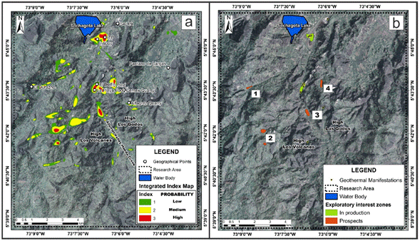
Figure 13 a) Integrated Index Map of Paipa Geothermal Zone. b) Explorations Prospects of Paipa Geothermal zone.
The four prospects were listed from one to four, and are located in: 1) El Durazno; 2) East of Alto Los Volcanes, divided into two circular anomalies; 3) Alluvial valley of the Honda creek, and 4) East of the El Delfín-La Playa pools.
Validation of Results
Surface Temperature
Surface temperature anomalies can be used with confidence once they have been appropriately validated. The approach used here includes the spatial comparison between surface temperature anomalies and soil temperature anomalies since the latter are a direct expression of the heat present in the subsoil. In general, five of the six soil temperature anomalies correspond spatially with satellite surface temperature anomalies (Figure 14a-1), demonstrating the geothermal component in thermal satellite images.
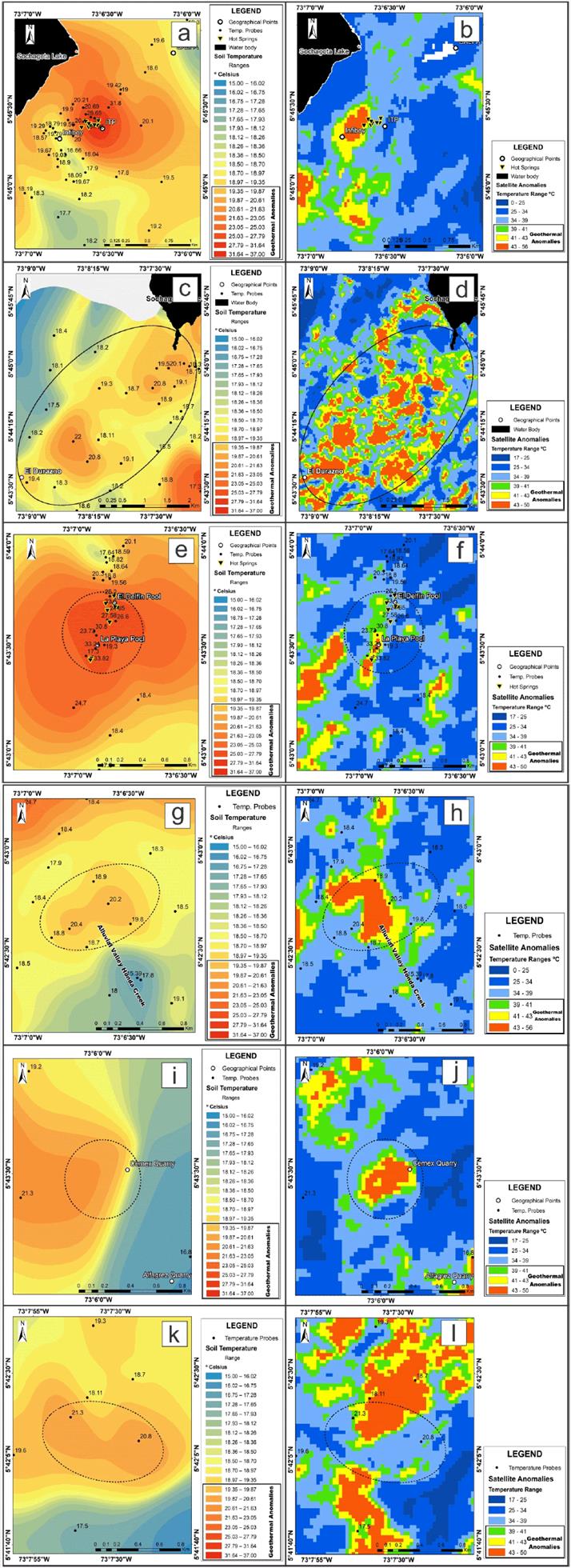
Figure 14 Spatial comparison of soil temperature anomalies and satellite temperature anomalies. a-b) Anomalies to the southeast of Lake Sochagota; c-d) Anomalies to the southwest of Lake Sochagota towards the Durazno sector; e-f) Anomalies to the sector of El Delfín and La Playa pools, where the presence of the second most important manifestations of the Paipa geothermal system occurs.
Exploratory Prospects
The results showed six areas of exploratory interest, two of which coincide spatially with the superficial geothermal manifestations of Paipa (Figure 13b). This spatial coincidence validates the results of the implemented method. The production area #1 (figure 15), is located in the main discharge area of the system, which contains approximately ten hot springs, with temperatures between 40°C and 72.1°C. These thermal waters are currently being used by the center Tourism (Instituto de Turismo de Paipa, ITP) and hotels in the area. Production area #2 (figure 16) corresponds with the second discharge area of the system. In this area, there are eight geothermal manifestations, of which seven are hot water springs and one steam vent (Alfaro Valero et al., 2017). The thermal waters register temperatures up to 60°C and are used in the El Delfín and La Playa pools. The steam vent registers a temperature of 64.6°C.
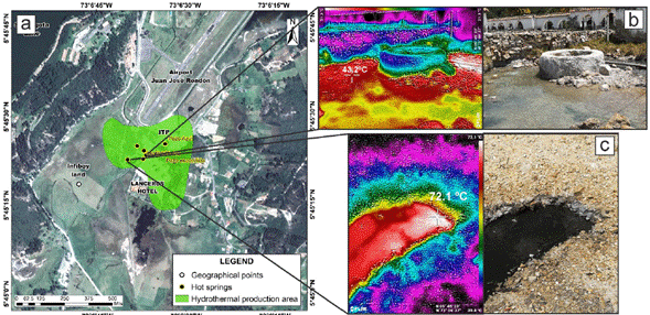
Figure 15 a) The spatial location of prospect #1 and hot springs in the main discharge area of the system (Infiboy-ITP). b) Thermal and visible photography of the Hot spring located next to the Hotel Lanceros; a maximum temperature of 51.3°C was recorded. c) Thermal and visible picture from the hot spring of the devil’s eye; a temperature of 72.1°C was registered.
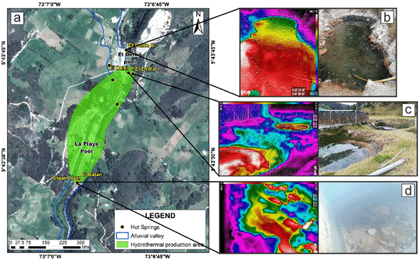
Figure 16 a) The spatial location of prospect #3 and hot springs in the second discharge area of the system (El Delfin-La Playa). b) Thermal and visible picture of the spring III El Delfín, it has a temperature of 54.1°C. c) Thermal and visible picture of hot springs I and II El Delfín. d) Thermal and visible picture of the steam vent in the La Playa sector; a maximum temperature of 64.6°C was registered.
Geological Context
Unlike geothermal reservoirs in active volcanic zones where thermal anomalies are located following a linear pattern according to the fault lineaments (Wu et al., 2012, Norini et al., 2015), the geothermal system of Paipa is different as the geothermal reservoirs are located through sedimentary rocks, which generates a lateral distribution of the hot fluids. The location of the thermal anomalies is found mainly to the northwest of the geothermal area (Figure 17a). This location can be a product of the circulation of hot fluids at shallow depth, through porous stratigraphic units of the Tilatá, Bogotá, Guaduas, Labor-Tierna, and Los Pinos formations, and facilitated by the faults, which function as migration paths. Figures 17aa and 17b show the El Batán overthrust fault, with a northeast course, of vergence towards the east, functioning as a limit (restricting), for the lateral circulation of hot fluids. The anomalies of surface temperatures found between the El Hornito and Canocas faults, southwest of Lake Sochagota (Figure 17a), would be validated, according to the conceptual geothermal model proposed by the CGS (Alfaro Valero et al., 2017), who proposed the existence of a secondary thermal system differing from the main one. This secondary system has a circulation of hot fluids at a shallow depth towards the northeast, by the porous sediments of the Guaduas and Bogotá formations.
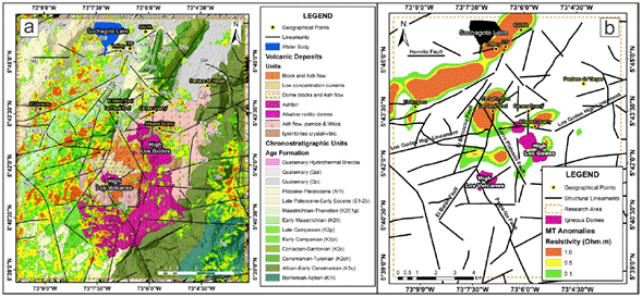
Figure 17 a) The spatial relationship between satellite thermal anomalies of Landsat 7 ETM+, from March 6, 2006, and surface geological formations; b) Spatial relationship between the anomalies of low resistivity (Magnetotelluric, Alfaro et al., 2017) and the lineaments of the research area.
Differently, for the thermal anomalies south of the Canocas fault, between the corridor generated by the faults the Bizcocho and the Batan, can be validated by the presence of hydrothermal fluids, inferred by the low resistivity anomalies (<1 Ω.m), obtained from the magnetotelluric technique at a height of 2,450 m.a.s.l, see figure 17b (Alfaro Valero et al., 2017). Other satellite thermal anomalies of smaller size (some coinciding with the Cerro Plateado fault on the alluvial deposits and others on volcanic deposits, east of the Alto Los Godos, coinciding with the Godos Lineament) have some spatial coincidence with low resistivity anomalies of the Magnetotelluric technique (Figure 17b). Finally, the satellite thermal anomalies present in the ITP-Infiboy and El Delfín-La Playa sectors are validated because they are present in the two zones where the only surface geothermal manifestations of the system are presented. These manifestations are produced through alluvial deposits, for the ITP-Infiboy sector facilitated by the crossing of the El Hornito and El Bizcocho faults, and for the El Delfín-La Playa sector, facilitated by the El Batán fault (Alfaro Valero et al., 2017).
Conclusions
This research used thermal infrared technology combined with conventional exploration methods to identify hydrothermal prospects in the Paipa geothermal region. Surface temperatures were obtained from the research area, from Landsat 7 ETM+ and Landsat 8 OLI/TIRS images. These images were calibrated and atmospherically corrected using the single channel and Split window algorithms, which led to spatially improved temperature anomalies being obtained. Additionally, fieldwork was carried out to validate satellite thermal anomalies. The fact that most satellite thermal anomalies coincide spatially with soil temperature anomalies validates the utility of satellite thermal bands in geothermal exploration. The spatial model implemented, determined six prospective areas of which two were validated by the spatial correlation of surface geothermal manifestations of the geothermal area of Paipa. The use of thermal satellite images for the correct identification of geothermal anomalies requires the incorporation of geological-geophysical analysis; this integration considerably improves the interpretation of satellite thermal information.

