


 English (pdf)
 Article in xml format
 Article references
 Send this article by e-mail
 Cited by SciELO
  Cited by Google
  Similars in
SciELO
Similars in
SciELO  Similars in Google
 Permalink
1. Introduction
The sediment bedrock morphology is an important geophysical interface for exploration of oil, gas, and mineral deposits. Under no compaction, a sedimentary cover is generally associated with negative gravity anomalies due to a low density of sediments in comparison to a surrounding rock density (Granser, 1987). Geophysical methods are often used to study the structure of sediment cover and underlying bedrock, most notably by applying seismic, gravimetric, and aeromagnetic methods as well as from drilling profiles.
The possibility of exploring mineral resources in the Southern Benue Trough (BT) in Nigeria has been of a high geological/geophysical interest over the last few decades. This has led to several aeromagnetic studies (e.g., Adebiyi et al, 2020; Obiora et al, 2018; Abdullahi et al, 2019; Opara et al., 2015; Oha et al., 2016; Obi et al., 2010; Ofoegbu and Onuoha, 1991; Ofoegbu, 1984; ) and gravimetric studies (e.g., Adighije, 1979; 1981a; 1981b; Cratchley and Jones, 1965; Ugbor and Okeke, 2010; Obasi et al., 2018; Omietimi et al., 2021) over parts of the region in order to ascertain its geological constituents in terms of residual anomalies, regional anomalies, trending lineaments, mineralization, and sediment thickness. Ofoegbu (1984) demonstrated that sediment depths between 1.7 and 7.3 km underlain the sedimentary cover in the Southern BT (which comprises the Lower and Middle BT). Ofoegbu and Onuoha (1991) estimated sediment depths to be between 1.3 and 2.5 km in the Abakaliki Anticlinorium within the Lower BT by applying a 2-D spectral analysis of aeromagnetic data. Obi et al. (2010) reported sediment depths between 1 and 4 km over parts of the Lower BT. Oha et al. (2016) estimated maximum sediment depths of 4.4 and 4.9 km for volcanic intrusions and basement respectively in parts of the Southern BT. The existence of deep magnetic source bodies (1.955.93 km) and shallow magnetic source bodies (0.1-1.8 km) was reported in several aeromagnetic studies (Adebiyi et al., 2020; Obiora et al., 2018; Opara et al., 2015). Adighije (1976; 1979; 1981a; 1981b) estimated the sediment thickness in the Southern BT by interpreting gravity data. He obtained an average sediment thickness of about 4.5 km (Adighije, 1976) and 4.25 km (Adighije, 1979) in the Lower BT. Adighije (1981a) pointed out that negative gravity anomalies flanking positive anomalies within the Middle and Lower BT could be associated with the accumulation of post-deformational cretaceous-tertiary sediments of lower density, which correspond with some smaller depositional basins such as the Anambra and Afikpo Basins. He obtained average sediment depths of 3.0 and 4.5 km in the Middle BT and the Lower BT respectively by using 2-D gravity profiles to fit geological models with gravity data. Obasi et al. (2018) reported the sediment thickness between 0.4 and 6.0 km beneath the Anambra Basin and its adjoining regions by applying a 2-D modelling of residual gravity data. The sediment thickness between 3.5 and 6.5 m within the Anambra Basin was detected by Omietimi et al. (2021) based on using a 2.5-D forward modelling along two selected profiles.
Adebiyi et al. (2020), Obiora et al. (2018), and Oha et al. (2016) suggested a possible reduction or absence of hydrocarbon accumulation in the Southern BT because of the dominance of intrusive bodies, which could hinder the thermal maturation of hydrocarbon and lead to over maturation of potential source rocks. The presence of hydrocarbon accumulation owing to the abundance of near-surface intrusive igneous rocks was proposed, for instance, by Agagu and Adighije (1983), Abdullahi et al. (2014), or Anyanwu and Mamah (2013). Although Ofoegbu and Onuoha (1991) revealed a suitable sediment depth for hydrocarbon generation, they finally agreed with the statement by Njoku (1985) and Whiteman (1982) on the unlikelihood of availability of hydrocarbon within the Abakaliki Anticlinorium due to its geological history. However, many of these studies (see Olade and Morton, 1985; Akande and Mucke, 1993; Onwuemesi and Egboka, 1989; Agumanu, 1989; Andrew-Oha et al., 2017; Abdullahi et al., 2019; Adebiyi et al., 2020) suggested an availability of other mineral sources, likely lead-zinc-copper-barium deposits within the Southern BT.
Most of existing studies dealing with the estimation of sediment thickness focused only on small portions of the Southern BT mainly because of an inadequate geophysical data coverage. Aeromagnetic studies concentrated on delineating directions of trending lineaments and fault lines (structural pattern) within parts of the Southern BT, while gravimetric studies used only a very irregular and sparse network of gravity measurements. To achieve a more comprehensive and concise gravimetric interpretation of the whole area, we estimated the sediment thickness over the entire Southern BT in Nigeria and parts of the Cameroon Volcanic Line (CVL) by employing the high-resolution synthetic gravity model prepared by Apeh and Tenzer (2022) in combination with geological evidence collected from 113 logged boreholes in order to validate our gravimetric inverse modelling results. The gravity inversion software GRV_D_inv, developed by Pharm et al. (2021a), was used to determine a 3-D depth structure of the basement relief. The GUI-based MATLAB software was successfully validated for practical applications and accuracy on both measured and synthetic gravity data, achieving a good fit between the computed and actual depth structures (Pham et al., 2021a).
2. Geological setting
The study area covering the Southern BT and parts of the CVL is a highly rifted region located between latitudes 4.98° to 8.31°N and longitudes 6.47° to 10.16°E (Fig. 1).
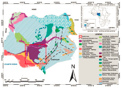
Figure 1 Location of the study area superposed on a generalized geological map of Nigeria (modified after Akpan et al. (2016) and Nguimbous-Kouoh et al. (2018)).
The Southern BT covers the Lower and Middle units of the Trough. The BT has been reported to have emanated from tensional fracture system with irregular subsidence along lines of weakness (Artsybashev and Kogbe, 1975). The Trough contains Cretaceous rocks whose ages date from the Middle Albian to Early Senonian epochs and filled with deltaic, estuarine, and marine sediments, with rare intrusions of basic alkaline lavas. The either side of the BT is bounded by granite and gneisses of probable lowermost Palaeozoic age, which make up the crystalline basement (Artsybashev and Kogbe, 1975).
Previous geophysical and geological studies (e.g., Nwachukwu, 1972; Reyment, 1965; Stoneley, 1966; Short and Stauble, 1967; Wright, 1968; Burke et al., 1972) revealed that the accumulation of Lower Cretaceous sediments (that is sedimentation) in Nigeria evolved along an elongated basin of subsidence in north-eastward direction which form the BT. Nwachukwu (1972) reported that the accumulation of sediments in the Southern part of the BT occurred through a series of marine transgressions and regressions beginning with the Albian transgression, which led to a formation of the Asu River group. A second phase of the sedimentation sequence formed the extensive Turonian transgression with deposits of the Ezeaku shales, which were later succeeded by the Awgu shales. The end of the Turonian was marked by a regressive phase, which was discontinued by the Maastrichtian transgression. A regressive phase within the southeast part of Nigeria occurred in Cenomanian, which hindered deposition of sediments to the Calabar flank (Nwachukwu, 1972). The youngest deformational episode in the BT was dated as Santonian whose folding may be closely associated with the undeformed coarsely crystalline sphalerite and galena in Abakaliki area (Nwachukwu, 1972). Odigi and Amajor (2009) attributed the sequence of sedimentation at the Lower BT to deformation events that led to longitudinal folds and faults of different orientations, dimensions, and styles.
Geological studies (e.g., Nwachukwu, 1972; Petters, 1978; Ofoegbu and Onuoha, 1991; Ojoh, 1992; Abbass and Mallam, 2013; Igwe et al., 2013; Abdullahi et al., 2019; Anudu et al., 2020; Apeh and Tenzer 2022) indicated the existence of ten major geological units in the Southern Benue Trough, consisting of the Asu River, Ezeaku, Awgu, Nkporo, Mamu, Ajali, Nsukka, Imo, Odukpani, and Precambrian basement. Studies also suggested that the Asu River group mostly comprises fractured shales and limestones with intercalations of sandstone within Abakaliki and Calabar Flank. The Ezeaku formation mainly consists of black shales, siltstones, and sandstones, while shales and limestones of the Coniacian age dominate the Awgu formation. Nkporo formations consist mainly of shales and mudstones. The Mamu formation comprises coals, while the Nsukka formation consists of carbonaceous shale, sandstones, and some thin coal seams. Fluvio-deltaic sandstones were deposited in the Ajali formation (Abbass and Mallam, 2013).
3. Input Data
3.1 Absolute gravity data
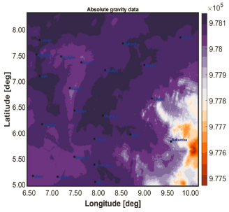
We prepared absolute gravity data on a 20x20" spherical grid (approximately 600 m) from the regional tailored (synthesized) absolute gravity model by following the approach developed by Apeh and Tenzer (2022). Their model was compiled by integrating the XGM2019e_2159 global gravity field model (Zingerle et al., 2019), terrestrial gravity data (NGSA, 2017), SRTM2gravity model (Hirt et al., 2019), and the Multi-Error-Removed Improved Terrain DEM (MERIT DEM) (Yamazaki et al, 2017) over the Southern BT. This synthetic gravity dataset was compiled by using a stochastic combination technique (Apeh and Tenzer, 2022). A validation of their tailored gravity model revealed a close fit with about 3000 sparse and irregularly spaced terrestrial gravity data over the Southern BT of Nigeria (Apeh and Tenzer, 2022). Spatial resolutions of 3"x3", 3"x3", and 5'x5' were utilized in the development of the MERIT DEM, SRTM2 gravity model, and XGM2019e_2159 global gravitational model respectively. The expected accuracy of the MERIT DEM heights is about 6 m (Yamazaki et al., 2017; Ebinne et al., 2022). For a more detailed explanation of how the model was developed and validated, we refer readers to the study by Apeh and Tenzer (2022).
In summary, topographic heights were extracted from the MERIT DEM on a 20x20" grid over the study area. The 20x20" grid data were used to subsequently extract the residual terrain gravity effects from the SRTM2gravity model (Hirt et al., 2019). Absolute gravity values were then computed on the MERIT topographic heights by using the XGM2019e_2159 global model available at the calculation service of the International Centre for Global Earth Models (ICGEM) online platform (Ince et al. 2019). The extracted residual terrain effects and a stochastically determined systematic bias of -0.4 mGal (Apeh and Tenzer, 2022) were algebraically added to the computed absolute gravity data to realize gravity data that fit a local gravity field. Figure 2 shows the map of the derived absolute gravity data which reflects mainly the topography and geological structure of the study area.
3.2 Logged borehole data
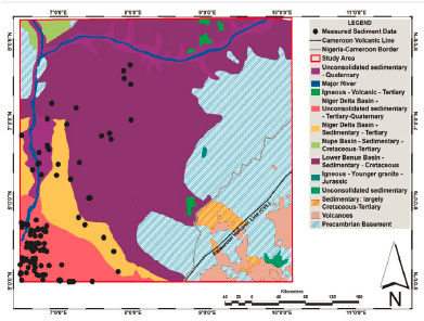
Many stratigraphic investigations of the study area were conducted by the government and private agencies as well as licenced oil companies. This has led to the availability of several wells log and borehole data within the Benue Trough and its environs especially in the southern parts of the Trough. The datasets were acquired by the Nigerian Upstream Regulatory Commission (NURC) and the Nigeria National Petroleum Corporation (NNPC), both governmental bodies in charge of all exploration activities across the country.
In this study, we used the geological information collected at 113 sites provided from the NNPC and its subsidiaries to validate results obtained from a gravity data inversion. These 113 logged boreholes were dug between years 1938 and 1996. Locations of these logged boreholes are identified in Figure 3. We note that since these 113 logged borehole sites are located at different locations, it is hardly possible to choose a density curve that varies with depth of sediments for the region. We further note that horizontal positions of these 113 logged boreholes were established using a local coordinate system mainly due to unavailability of Global Navigation Satellite Systems (GNSS) at that time. This may slightly affect the accuracy of their locations or lead to some inaccuracies of their exact horizontal positions after conversion to geographic coordinates.
3.3 CRUST1.0 and GEMMA sediment thickness
For the sake of comparative assessment, we extracted the sediment thickness from the CRUST1.0 (Laske et al., 2013) and GEMMA (Reguzzoni and Sampietro, 2015) global crustal models at the study area. The CRUST1.0 global seismic crustal model consists of ice, seawater, sediments and consolidated (crystalline) crustal layers data on a 1x1° grid. Authors of the CRUST1.0 seismic model used global datasets obtained from active seismic methods and deep drilling profiles to prepare the sediment and crustal structures in regions where no seismic measurements were available. The GEMMA gravimetric model was prepared on a 0.5x0.5° global grid by employing the GOCE gravity gradiometry observables (Drinkwater et al., 2006; Migliaccio et al. , 2011) and globally averaged data from active seismic surveys. The maps of sediment thickness obtained from these two global crustal models with their relevant statistics and interpretations are provided in Section 5.
4. Methods
4.1 Gravimetric inversion
The model space can be described in a 3-D Cartesian coordinate system such that the axes x, y, and z point towards east, north, and positive downwards respectively. A 3-D mathematical expression of a gravity data in the Fourier domain is given in the following form (Parker, 1973; Gao and Sun, 2019; Pham et al. 2021a)
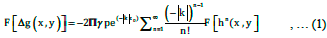
where p is the density contrast, γ is the Newton's gravitational constant, h is the interface topography at the reference depth zo, F[] denotes the Fourier transform operator, and  , with k
x
and k
y
denoting the wave-numbers along the plane direction.
, with k
x
and k
y
denoting the wave-numbers along the plane direction.
The rearrangement of Equation 1 gives
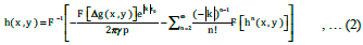
where F-1 is the inverse Fourier Transform.
The expression in Equation 2 is solved iteratively to estimate the depth to density interface, while using the RMS of differences (Pham et al., 2021a) to measure the fitting between two successive depth estimates. To ensure the convergence of Equation 2, a low-pass filter is normally applied during the calculation. The filter is defined in the following form
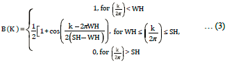
where WH and SH describe smaller and greater roll-off frequencies of the filter design. This filter cuts off the frequencies higher than SH and fully passes the frequencies greater than WH while attenuating between WH and SH. The parameters of the roll-off frequencies can be determined from a spectral analysis of gravity data.
The initial model is obtained from Equation 2. Here, the first term of Equation 2 is computed by assigning h (x, y) = 0 and its inverse Fourier transform provides the first approximation of the topographic interface, h (x, y). This value of h (x, y) is then used in Equation 2 to evaluate a new estimate of h (x, y). This process is continued until a reasonable solution (in terms of existing geological/geophysical information) is achieved.
4.2 Determination of a 3-D basement relief
We computed the complete Bouguer gravity data by utilizing gravity reduction techniques and applying the well-known crustal density value of 2.67 gcm-3 (Heiskanen & Moritz, 1967). We note here that terrain gravity effects are part of the residual gravity effects obtained from the SRTM2gravity model and hence there is no need to compute and add terrain corrections anymore (Hirt et al., 2019; Apeh and Tenzer, 2022). The result of the complete Bouguer gravity data is shown in Section 5.1.
We then used an algorithm for an optimum upward continuation height developed by Zeng et al. (2007) to separate the residual and regional gravity signals in the complete Bouguer gravity data. This technique designs a scheme of computing a best height for the upward continuation in order to carry out the regional-residual gravity separation. The method of Zeng et al. (2007) uses the cross-correlation between original data and the upward continued signal to determine the 'optimal' upward continuation distance for isolating a localized signal hidden inside a regional trend.
Figure 4 shows the cross-correlation between continuations to two successive heights versus the height (Fig. 4a) and the deflection C versus the height (Fig. 4b). As shown in Figure 4b, the curve of the deflection against height shows maximum at the height of 10 km being regarded as optimal. The red line in Figure 4a shows the chord connecting the starting point to the end point of the height values (Zeng et al., 2007).
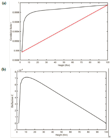
Figure 4 (a) Cross-correlations between continuations to two successive heights versus the height. (b) The deflection C versus the height. The red line in Figure 4a shows the chord joining the starting and end points of the height values.
As aforenoted, 113 sediment thickness measurements were used to validate results of a 3-D inverse modelling of the sediment thickness from the residual gravity data. Given that the accuracy of sediment thickness estimates depends on parameters of density contrast and mean sediment depth (see Eqs 1-3), we used the density contrast values between 0.11 and 0.37 gcm-3 with a step of 0.02 gcm-3 and the mean sediment depths between 0 and 3.6 km with a step of 0.3 km. As already noted, the 113 logged boreholes are at different locations and hence, it is hardly possible to choose a density curve that varies with depth of sediment for the region. We numerically computed and evaluated the resulting sediment thickness from the MATLAB-based 3-D gravity modelling program (described in Section 4.1) by using varying density contrasts and mean sediment depths until we got the minimum RMS of differences between computed and measured (borehole-derived) sediment thickness data.
We selected the range of density contrasts and mean sediment depths based on previous studies and density measurements within and around the study area. Agagu and Adighije (1983) used the sediment density contrast of 0.17 gcm-3 to estimate the sediment thickness of two profiles running from Auchi-Gboko and Lokoja-Abakaliki. Fairhead et al. (1991) used the value of 0.2 gcm-3 for density contrast to carry out a 2-D interpretation of sediments in the Mamfe Basin located in West Africa. Obasi et al. (2018) and Omietimi et al. (2021) applied 2.4 gcm-3 and 2.7 gcm-3 as the mean densities (which implies a mean density contrast of 0.3 gcm-3) of the sedimentary and basement layers respectively in their studies. Adighije (1981b) collected 46 core samples of sedimentary rocks within the Lower BT for density measurements. He first weighed samples in air and then saturated them in water to obtain mean densities of 2.65±0.04, 2.48±0.05, 2.45±0.05, 2.53±0.02, and 2.3±0.09 gcm-3 for the Albian shales, Cenomanian Sandstone, Turonian-Senonian Sandstone, Turonian-Senonian Shale, and Maastrichtian-Tertiary Sandstone respectively. In a similar study by Cratchley and Jones (1965), 2.65, 2.48, 2.53 and 2.45 gcm-3 density values were obtained for the Albian shales, Cenomanian shale, Turonian-Senonian shale, and Turonian-Senonian sandstone respectively. Adighije (1981b) used the average density of 2.53±0.12 gcm-3 to obtain a simple model of the sediment thickness within the Lower BT. Adighije (1981b) subsequently collected 157 samples of basement complex rocks, mainly migmatites. He obtained the mean density of 2.7±0.07 gcm3. Based on his measurements, he stated that a density contrast between basement and sediments might possibly vary from 0.15 to 0.25 gcm-3.
5. Results and Discussion
5.1 Gravity reduction and separation
The maps of the complete Bouguer gravity data (Fig. 5a), residual Bouguer gravity data (Fig. 5b) and the regional Bouguer gravity data (Fig. 5c) are shown in Figure 5. We note that positive gravity anomalies were not completely separated from negative anomalies because of the complexity of the geological setting of the study area. We used the method by Zeng et al. (2007) as described in section 4.2 to carry out the Regional-Residual gravity separation at the optimal height of 10 km.
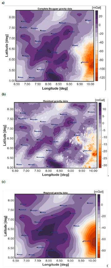
Figure 5 Gravity maps of: (a) the complete Bouguer gravity data, (b) the residual gravity data, and (c) the regional gravity data over the study area
The Bouguer gravity map, shown in Figure 5a, depicts both, positive and negative anomalies ranging from -122 to 33 mGal. The Bouguer gravity pattern exhibits continuities as well as discontinuities of rifting within the entire study area. We could see a notable zone of positive anomaly bounded by negative anomalies on both sides. Towards the south and middle parts of the study area, we recognize a gravity pattern associated with the Precambrian basement rocks, with low-density bodies at the Lower BT dominating the southwest part of the study area and the flexurally inverted and circular Abakaliki Anticlinorium towards the central part of the study area.
We could see negative anomalies flanking positive anomalies especially in the residual gravity map (Fig. 5b). These positive anomalies are mainly trending from the central portion towards southeastern part of the study area. The negative anomalies appear to correspond with several smaller well-known depositional basins, such as Ankpa, Onitsha and Afikpo, which are filled up with Cretaceous-Tertiary sediments. It is commonly assumed that the negative Bouguer gravity anomalies are largely attributed to relatively low-density sediments occurring in the basin and lie on top of the metamorphic basement rocks that are of higher density. We could infer from the gravity maps (Figs. 5a, b, c), based on the presence of alternating gravity lows and highs, that the Benue Trough may have resulted from uplift, rifting, subsidence, and sedimentation. According to a study by Odigi and Amajor (2009), "the sedimentary sequence of the Lower BT is said to be affected by two well-documented deformation episodes, namely the Cenomanian and Santonian episodes, which resulted in longitudinal folds and faults of varying styles, orientations, and dimensions". We note that the most pronounced negative anomalies towards the southeastern part of the study area correlate with a topographic high, which is likely a crustal-root exhibiting isostasy.
The regional gravity map (Fig. 5c) portrays a kind of magmatic movements giving rise to the alternating positive and negative gravity values prevalent within the study area. There is a possible existence of a high-density material giving rise to the positive values in the residual positive gravity data (see Fig. 5b) which tend to decrease in width and thickness from the southern to the north-eastern end of the study area. The region of residual positive anomaly (at the central portion) extends steadily from southwest to northeast and matches with the core of the Abakaliki anticlinorium where the Albian shales connect with several mafic intrusive and basaltic rocks as noted by Olade (1976). The positive anomaly seems to disappear around latitude 90 N as confirmed by Adighije (1979; 1981a; 1981b).
The gravity maps (Figs. 5a, b, c) show positive values over the northwest and southeast portions of the study area underlain by the crystalline basement rocks (see Fig. 1). These positive anomalies may be attributed to the intra-sedimentary volcanic rocks and/or to basement deformations in horst and graben structures, while the low amplitude anomalies could be due to the Cretaceous sedimentary rocks (see Fig. 1). The gravity maps also revealed the presence of many intra-sedimentary volcanic rocks and varying geological structures (faults, folds, synclines, anticlines, massifs or highlands) corresponding to some known and formerly unknown features in previous studies (e.g., Nwachukwu, 1972; Odigi and Amajor, 2009; Anudu et al., 2020). The prevalence of igneous intrusions (associated with the positive gravity values) within the study area may have led to serious fracturing and faulting of the basement, and overlying sediments. Resulting geological structures from these tectonic events could make way for hydrothermal fluid migration and accumulation of mineral resources (Ekwok et al., 2022). Usually, magmatic movements (as seen especially within the Abakaliki area) could help segregate minor elements of the magma from the major elements and concentrate them in some smaller volumes of rocks. These magmatic processes may form mineral deposits mainly associated with igneous intrusions resulting from rifting and volcanic activities.
5.2 Selection of optimal parameters
We used spectral analysis of the residual gravity data to determine the parameters of the roll-off frequencies (WH and SH). The power spectrum of the residual gravity data and the marked frequencies of WH (in blue colour) and SH (in red colour) are demonstrated in Figure 6. We used the values WH= 0.025614 and SH= 0.050418 as the cut-off or roll-off frequencies. Broadly speaking, low radial wavenumbers mostly correspond to deep sources, and intermediate wavenumbers mainly relate to sources having average depth, while high wavenumbers are dominated by very shallow ones and noise (e.g., Pham et al., 2020; Spector and Grant, 1970). To ensure the convergence of the algorithm, we chose a cut-off frequency SH of 0.05 and the frequency WH equal to half of SH (WH = 0.5SH) as reported by Caratori Tontini et al. (2008) and Pham et al. (2020, 2021b).
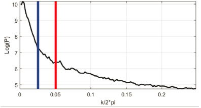
Figure 6 Power spectrum of the residual gravity data with marked cut-off frequencies. WH (in blue colour) and SH (in red colour) describe smaller and greater roll-off frequencies of the filter design.
We computed the predicted inversion results 156 times and compared them with the 113 measured sediment depths to determine the mean density contrast and sediment depth for the entire study area. Unfortunately, we do not have data that could empirically describe the porosity change with depth (or the sediment density change with depth) that can be used to determine if the sediment thickness increases significantly due to compaction. Hence, we assumed only a constant sediment density as stochastically obtained from the gravity inversion performed 156 times to determine the optimal value in relation with the available measured sediment data. The RMS of residuals between the computed and measured sediment depths (which ranges from 0.8 to 2.95 km) are given in Table 1. The computed sediment depths are based on density contrasts (which range from 0.11 to 0.37 gcm-3) and mean sediment depths (which range from 0 to 3.6 km).
Table 1 RMS of residuals between measured and computed sediment depths based on density contrasts and mean sediment depths.
| Mean sediment depths (km) | Density contrasts (gcm-3) | |||||||||||||
| 0.11 | 0.13 | 0.15 | 0.17 | 0.19 | 0.21 | 0.23 | 0.25 | 0.27 | 0.29 | 0.31 | 0.33 | 0.35 | 0.37 | |
| RMS of residuals | ||||||||||||||
| 0.0 | 2.73 | 2.77 | 2.81 | 2.83 | 2.86 | 2.88 | 2.89 | 2.9 | 2.92 | 2.93 | 2.94 | 2.94 | 2.95 | 2.96 |
| 0.3 | 2.44 | 2.48 | 2.52 | 2.54 | 2.57 | 2.58 | 2.6 | 2.61 | 2.63 | 2.64 | 2.65 | 2.65 | 2.66 | 2.67 |
| 0.6 | 2.16 | 2.20 | 2.23 | 2.26 | 2.28 | 2.30 | 2.31 | 2.33 | 2.34 | 2.35 | 2.36 | 2.37 | 2.38 | 2.38 |
| 0.9 | 1.89 | 1.92 | 1.95 | 1.98 | 2.00 | 2.02 | 2.03 | 2.05 | 2.06 | 2.07 | 2.08 | 2.09 | 2.09 | 2.10 |
| 1.2 | 1.62 | 1.65 | 1.68 | 1.70 | 1.72 | 1.74 | 1.76 | 1.77 | 1.78 | 1.79 | 1.8 | 1.81 | 1.82 | 1.83 |
| 1.5 | 1.38 | 1.40 | 1.42 | 1.44 | 1.46 | 1.48 | 1.49 | 1.51 | 1.52 | 1.53 | 1.54 | 1.55 | 1.55 | 1.56 |
| 1.8 | 1.17 | 1.17 | 1.19 | 1.20 | 1.22 | 1.23 | 1.25 | 1.26 | 1.27 | 1.28 | 1.29 | 1.30 | 1.31 | 1.31 |
| 2.1 | 1.01 | 0.99 | 0.99 | 1.00 | 1.01 | 1.02 | 1.03 | 1.04 | 1.05 | 1.06 | 1.07 | 1.08 | 1.08 | 1.09 |
| 2.4 | 0.92 | 0.88 | 0.87 | 0.86 | 0.86 | 0.87 | 0.87 | 0.88 | 0.89 | 0.89 | 0.9 | 0.91 | 0.91 | 0.92 |
| 2.7 | 0.94 | 0.87 | 0.84 | 0.82 | 0.81 | 0.80 | 0.80 | 0.80 | 0.81 | 0.81 | 0.81 | 0.81 | 0.82 | 0.82 |
| 3.0 | 1.05 | 0.97 | 0.92 | 0.89 | 0.87 | 0.85 | 0.84 | 0.84 | 0.83 | 0.83 | 0.83 | 0.83 | 0.83 | 0.83 |
| 3.3 | 1.23 | 1.14 | 1.08 | 1.04 | 1.01 | 0.99 | 0.98 | 0.97 | 0.96 | 0.96 | 0.95 | 0.95 | 0.95 | 0.94 |
| 3.6 | 1.46 | 1.36 | 1.30 | 1.25 | 1.22 | 1.20 | 1.18 | 1.17 | 1.16 | 1.15 | 1.14 | 1.14 | 1.13 | 1.13 |
As seen in Table 1, the mean sediment depth of 2.7 km most suitably represents the statistics obtained from the measured sediment depths. One could infer from the presented statistics that the density contrasts of 0.21, 0.23, and 0.25 gcm-3 have the best RMS fit. To determine the best density contrast to be used, we averaged these three density contrasts with the best RMS fit and obtained the value of 0.23 gcm-3. Following these statistical analyses, we selected the density contrast of 0.23±0.02 gcm-3 and the mean sediment depth of 2.7 km as numerically optimal values for the estimation of sediment thickness. We clarify here that our numerically obtained density contrast is within the given range of Cretaceous to tertiary sediments from other studies (Adighije, 1981a, b; Cratchley and Jones, 1965; Rotstein et al., 2006). Adighije (1981a, b) and Cratchley and Jones (1965) revealed a mean density range of 2.30-2.65 gcm-3 from about 46 samples of sediments within the study area. Adighije (1981b) demonstrated that the sediment-basement density contrast within the LBT could vary between 0.15 and 0.25 gcm-3. Elsewhere, Rotstein et al. (2006) revealed a density variation of 2.35-2.45 gcm-3 for tertiary rift sediments at the Upper Rhine Graben in Germany.
5.3 Sediment thickness
We used optimal values of the density contrast (0.23 gcm-3) and the mean sediment depth (2.7 km) to estimate the sediment thicknesses. The result is shown in Figure 7.
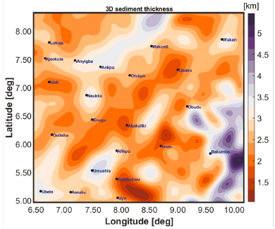
Figure 7 Sediment thickness map derived from the density contrast of 0.23 gcm-3 and the mean sediment depth of 2.7 km.
The obtained sediment depths exhibit the complexity of the Southern BT and adjacent regions. Intrusive rocks with lower sediment depths are prevalent within the study area. These intrusive rocks are mainly seen along NE-SW direction justifying the well-documented NE-SW direction of the rift system (Olade, 1975). Adighije (1981b) posited that the intrusive rocks are mainly syenitic, dioritic, and gabbroic in composition and are generally intermediate to basic in character. Field investigations reveal diorites and dolerite as usual igneous rocks found within the Abakaliki area (Obiora and Charan, 2010). The sediment thickness sections along the Abakaliki Anticlinorium are typically less than 1.7 km, probably due to a combination of uplift (upwelling of the crust) and erosion. Farrington (1952) and Olade (1975) averred that the zone of positive anomaly is limited to the regions of where tectonic activity, mineralization, uplift, and erosion are prevalent within the Trough.
It is evident that the sediments in the southwest part of the Trough are thicker than on the eastern side except for a portion around the Cameroon Volcanic Line. This could be explained by the proximity of the southwest part of the study area to the Atlantic Ocean, the Niger Delta, and the low-lying topography of the region. The zones of positive anomaly (over and around the towns named Abakaliki, Gboko, Arochukwu and Ikom, in Figure 5) correspond with areas of shallow depth of basement and hence, low sediment depth. We could see a maximum of about 4500 m sediment thickness within the Southwestern end. Similarly, Adighije (1981a, 1981b) reported the maximum sediment thickness of 4500 m around Nsukka and 5000 m around the Ankpa Basin, while Kogbe (1976) estimated the maximum sediment thickness of3300 m for the Albian-Coniacian sediments within the Lower Benue Trough from surface geology. Agagu and Adighije (1983) pointed out that the variations of sediment thicknesses in the Lower BT could be associated with some known tectonic events, namely: (a) Abakaliki High, (b) Nsukka High, (c) Ankpa Basin, (d) Onitsha Basin and (e) Afikpo Syncline. These well-known tectonic events as observed by Agagu and Adighije (1983) are clearly delineated in Figure 7.
The South-western part of the study area (part of Niger Delta in Nigeria) with deep sediments is well-known for oil and gas exploration and exploitation activities. There is a recent discovery of oil and gas within the Anambra Basin around the town indicated as Onitsha in Figure 7. More exploration activities could lead to a discovery of other liquid and solid mineral resources around the places where deep sediments are detected in Figure 7. Magmatic movements or processes along and over the Abakaliki Anticlinorium may have led to the shallowing of sediments over that portion of the study area. There is the likelihood of sediments been entrapped within and under the basement complex, which could mature overtime into mineral resources.
5.4.1 Comparison of results
The differences between our gravimetrically determined sediment depths and that of the 113 logged (measured) borehole data are demonstrated in Figure 8. These differences range from -2.38 to 1.50 km with some few locations not fitting well. However, it is obvious that most of the differences are within ±0.5 km.
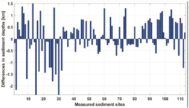
Relatively large differences in some few locations could be attributed to a possible shift in their geographic position during coordinate transformation, uncertainties in the gravimetric inversion parameters, variable geology, and lithology. We used the geographic coordinates of the boreholes to extract sediment depths from our 3D sediment thickness data. A more explanation of these differences is given in section 5.5.
The maps of sediment depths extracted from the CRUST1.0 (Fig. 9a) and the GEMMA (Fig. 9b) are presented in Figure 9, with statistics in Table 2. We compared the CRUST1.0, GEMMA, and our gravimetric sediment thickness estimates with the measured values (logged borehole data). Statistics of differences are given in Table 3. We clarify that the global models have a lower resolution compared to our sediment data. However, the comparison could help justify our gravity tailoring and gravimetric inversion efforts. It also shows that despite the differences between our gravimetrically determined and measured sediment depths, our result is far better than gridding and using those global sediment models over such a geologically complex study area. Within the study area, the CRUST1.0 sediment thickness ranges from 0 km to 10.3 km, and the GEMMA sediment thickness is from 0 to 10.2 km.
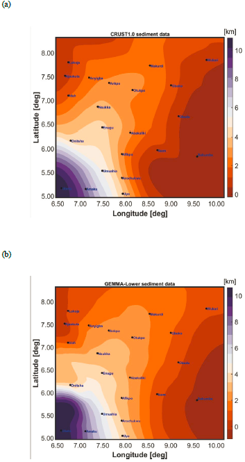
Table 2 Statistics of 113 sediment depths obtained from different models
| Models | MIN (km) | MAX (km) | MEAN (km) | STD (km) |
|---|---|---|---|---|
| Measured sediment depths | 0.102 | 4.506 | 2.948 | 0.887 |
| Sediment depths obtained using our gravimetric model | 1.792 | 3.656 | 2.903 | 0.394 |
| Sediment depths obtained using CRUST1.0 model | 1.775 | 8.980 | 6.546 | 2.034 |
| Sediment depths obtained using GEMMA model | 0.565 | 9.985 | 7.716 | 3.123 |
Table 3 Statistics of the residuals between the computed and measured sediment depths
| Models | MIN (km) | MAX (km) | MEAN (km) | RMS (km) |
|---|---|---|---|---|
| Our gravimetric model | -2.378 | 1.504 | 0.045 | 0.803 |
| CRUST1.0 model | -6.421 | 1.205 | -3.598 | 4.010 |
| GEMMA model | -7.672 | 2.490 | -4.768 | 5.491 |
Not surprisingly, our gravimetrically estimated sediment thickness is moderately consistent with the measured sediment depths from logged boreholes without a significant systematic bias as our result was fitted with these values. Both global models are more consistent with each other but significantly differ from our results and logged borehole data. Unlike our sediment thickness estimates (Fig. 7), the CRUST1.0 and GEMMA sediment thickness less than 2 km are seen towards the eastern part of the study area. This could be due to a sparse geophysical data coverage and spatial resolution of those global models. The two models overestimate the sediment thickness towards the southwest part of the study area, while underestimating it elsewhere. Consequently, the use of these global models within the study area for geophysical investigations might bring an overestimation of geological/geophysical features in the region which could lead to biased interpretations and conclusions. The moderate correlation of the gravimetrically computed sediment data with the measured sediment data, on the other hand, justifies the need to estimate sediment thickness from high-resolution gravity data.
5.5 Uncertainties and limitations of the inversion results
The uncertainty in the chosen density contrast (0.23±0.02 gcm-3) translates to about 20% uncertainty of the inverted thickness map as well as uncertainties arising from the logging of the boreholes to determine sediment depths. Hence, the true range of acceptable density contrasts within the study could be even wider.
Owing to compaction and variable geology, the assumption of a constant density contrast might not be ideal for sediments, especially where thickness varies significantly, as it does in our study area. This could be a major limitation of the two-layer approach with the assumption of a simple density contrast. For very thick sediments, the presence of a density contrast between the sedimentary and basement rocks is questionable due to compaction. In another vein, the coverage of the borehole data is not evenly distributed over the study area. The concentration of boreholes in the southwest part of the study area is explained by the major focus on exploration and exploitation of mineral resources (such as oil and gas) in Nigeria. As already aforenoted, there could be some inaccuracies in horizontal positions of the boreholes due to errors arising from a coordinate transformation from local to geographic system. In trying to enhance the relative accuracy of the density contrast used in this study, we computed the predicted inversion results 156 times and compared them with the 113 measured sediment depths to determine the mean density contrast and sediment depth for the entire study area. Hence, we assumed the mean constant density of 0.23 gcm-3 as stochastically obtained from the gravity inversion performed 156 times to determine the optimal value in relation with the available measured sediment data.
It is obvious that the exposed basement in the southeast part of the study area is recovered as thickened sediments to explain the negative anomaly. As mentioned earlier, the negative anomaly correlates with an elevated topography and so, it is likely a crustal root exhibiting isostatic reactions to the volcanic activities taking place over there. We note that the regional-residual gravity separation did not separate completely the regional field from the residual field mainly because of the geological and tectonic complexity of the study area. As a result, it is obvious that the regional field contains sedimentary signal, and the residual field contains deeper signals.
6. Conclusions
Authors compiled the map of sediment thickness for the Southern Benue Trough and parts of the Cameroon Volcanic Line by applying a 3-D gravimetric inversion of a high-resolution tailored gravity data validated by wells log and borehole data. We used a gravity separation method to remove the residual gravity signature from the regional gravity trend. A 3-D gravimetric inversion of the residual gravity data was performed, and a numerical modelling procedure was carried out on the gravimetrically inverted sediment depths in order to obtain optimal values for the density contrast and the mean sediment depth. The optimal density contrast of 0.23 gcm-3 and the mean sediment depth of 2.7 km were statistically realized.
Our gravity maps closely mimic the geological configuration of the study area. The gravity maps revealed the prevalence of igneous intrusions, which might have led to serious fracturing and faulting of the basement, and overlying sediments. Magmatic processes showing potential for hydrothermal fluid migration and mineralization accumulation are recognizable. These magmatic processes/movements are seen as positive anomalies in the presented gravity maps (Figs. 5a, b, c).
According to our estimates, the 3-D depth structure of the basement relief (sediment thickness) within this geologically and tectonically complex region range from 0.8 to 5.5 km. The sediment thickness increases westerly and decreases easterly, demonstrating the various tectonic events within the study area, which are consistent with previous studies. The sediment thickness sections along and over the Abakaliki Anticlinorium are small probably due to a combination of uplift (upwelling of the crust) and erosion. Our gravimetrically inverted sediment depths have almost no systematic bias with measured sediment data unlike large systematic biases found when using the CRUST1.0 and GEMMA global models. This implies that our approach of acquiring high-resolution gravity data and subsequent modelling processes to compute sediment data could be beneficial for many developing countries and regions with insufficient coverage of logged borehole data.
Most parts of the Southern Benue Trough, where deep sediments are located, are well-known for oil and gas exploration and exploitation activities. Other liquid and solid mineral resources may be present in and around those places. We speculate that large magmatic movements or processes along the Abakaliki Anticlinorium, which led to the shallowing of sediments over that portion of the study area, might have entrapped enough sediments suitable for maturation of mineral resources overtime.

