1. Introduction

According to ^{Flores et al. (2012)}, the area in the state of Sinaloa is predominantly classified as subtropical-intertropical, with zones of low topographic relief near the Pacific Ocean and extreme elevations in the mountain system known as the Sierra Madre Occidental. The climatic variability-randomness of this area can be numerically modeled using criteria based on significant trends (ST), adjusted return periods (ARP) and fitted probability distribution functions (^{Cohen et al., 2012}; ^{Rustom 2012}; ^{Franzke 2015}; ^{Kienzle 2018}; ^{Chapman et al., 2019}; ^{Garry et al., 2019}; ^{Latif & Mustafa 2020}; ^{Alves et al., 2021}). These mathematical tools were used to characterize the climate variability (^{Llanes et al., 2022b}; Llanes, 2023) and randomness of Sinaloa; i.e., indicators of hot extremes (HE, Llanes et al., 2022a), since determination of the STs can be helpful for identifying zones where extreme climate changes occur, and knowledge about such changes has been demonstrated to be very useful for designing adaptation/prevention strategies to face natural disasters (^{Blanco et al., 2014}). Globally, the HE maximum maximorum (highest maximum) temperatures (MmT) are some of the most important indicators of change climate and can provide valuable information about the climate conditions to which the crops in a region are subjected (^{Li et al., 2018}; ^{Ruiz et al., 2005}). The major crops produced in the area of Sinaloa state, nicknamed "the breadbasket of Mexico" (^{Rincón 2012}), are maize, sorghum, wheat, and beans, which are particularly vulnerable to temperature extremes and droughts (SAGARPA 2015; ^{Gudko et al., 2021}; ^{Gurung et al., 2021}; ^{Habibi & Meddi 2021}). The negative effects of a high frequency of maximum extreme temperature (MeT) events can include human deaths as a consequence of gastrointestinal diseases and heat stroke (^{Murage et al., 2017}; OPS 2019).

With ARPs, the indicators of climate extremes can be estimated with very low uncertainty and the highest efficiency and reliability (^{Aguilera 2007}; ^{Campos 2014}; ^{Lustenberger et al., 2014}; ^{Deng & Zhu 2021}). Worldwide, there are multiple studies that address ST using non-parametric Mann-Kendall tests (^{Kumar et al., 2023}), as well as the use of fitted probability distribution functions, due principally to the importance, reliability, and efficiency of modeling (^{González et al., 2011}; ^{Fontanelli et al., 2019}).

In this study, based on HE indicators (^{Li et al., 2018}) of the MeT and MmT (^{Ruiz et al., 2005}), the negative climate effects in Sinaloa were calculated according to the criteria established by Li et al. (2018). According to ^{Wang et al. (2016)} and ^{Hochman et al. (2022)}, many studies indicate that extreme climate events may intensify or become more frequent and long-lasting with climate change, especially in semi-arid regions (^{Demisse et al., 2022}) such as the state of Sinaloa (^{Llanes et al., 2022b}). Due to the high interconnection with drought (^{Horton et al., 2016}; ^{Yuan et al., 2016}), the HE indicators calculated were frequency (FR), annual average duration (AAD), annual daily duration (ADD) and intensity (IN) (^{Seneviratne et al., 2012}).

To learn about previous research related to this study, a review was done of the literature (documents available locally and worldwide). ^{Jaiswal et al. (2023)} calculated extreme climate indices in India (hot days and daily maximum temperature) and ^{Llanes et al. (2022a)} calculated indicators of MeT (HE and MmT) in Sinaloa, but did not calculate their trends or return periods through fitted probability distribution functions.

The modeling tools of this study (ST, fitted probability distribution functions and ARP) provide a new method to estimate the frequency of occurrence of MeT indicators HE (FR, AAD, ADD and IN) and MmT. This method can help to prevent impacts on agricultural yields through climate-smart practices such as drip irrigation, conservation agriculture, precision fertilization, protected agriculture, and crop substitution, which will withstand future hot temperature extremes (World Bank et al., 2014), not only in Sinaloa, but throughout Mexico. For this reason, the goal of this investigation was to calculate MeT indicators based on STs and ARPs, to design climate-smart agricultural adaptation/prevention strategies.

2. Material and methods

2.1 Study area

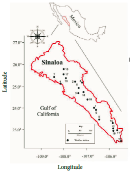
The state of Sinaloa is located between 105° 23' 32" and 109° 26' 52" N, and 27° 02' 32" and 22° 28' 02" W (Figure 1). It comprises approximately 2.9% of the total territory of the country (INEGI 2016).

Figure 1 Location of the study area. State of Sinaloa Source: ^{Llanes et al. (2021)}  

2.2 Data collection and processing

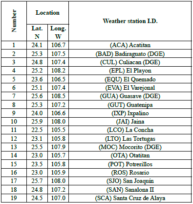
Daily maximum temperature data for April-October were obtained for 19 weather stations in the study area from the CLImate COMputing database (CLICOM, 2021) at the website http://clicom-mex.cicese.mx/mapa.html for the period 1982-2014 (Table 1). Missing data were estimated though the multiple imputation method (^{Little & Rubin, 1987}) with the Markov chain Monte Carlo algorithm (MCMC; ^{Austin & Van Buuren, 2022}) since, according to ^{Puerta (2002)} and ^{Salgado & Largo (2018)}, with this method it is possible to obtain unbiased estimators that can be used efficiently. For this calculation, the XLstat version 2014 program was used. This program works in the Windows Excel environment and is widely used worldwide in climatology. These data were obtained from ^{Llanes et al. (2021)}

Table 1 Location of the weather stations. 

HE indicators and MmT

To obtain some of the most important variables used worldwide to characterize extreme weather, the following HE indicators were calculated following ^{Li's method (Li et al., 2018}): FR, AAD, ADD and IN. These authors define a HE event as occurring when the value of daily maximum temperature exceeds the 85^th and 90^th percentiles (P85 and P90, respectively) for three consecutive days (Stefanon et al., 2012, Zschenderlein et al., 2019 and ^{Llanes et al., 2022a}). The values of MmT were obtained according to ^{Ruiz et al. (2005)}, who defined these variables as the maximum monthly value in a series of maximum daily temperatures. To calculate the HE indicators and MmT, the XLstat version 2014 program was used. The authors used the data of the HE indicators FR, AAD, ADD and IN, previously calculated by Llanes et al. (2022a).

ST of MeT indicators

In order to determine whether local climate trends are cooling or warming, the STs of the annual average values of FR, AAD, ADD, IN and MmT were calculated.

The ^{Mann-Kendall test for trend analysis (Mann, 1945}; Kendall, 1975, Table 2) and ^{Sen's slope test (Sen 1968)} for magnitude of trend (Figure 3) were applied. To identify the presence of STs of MeT indicators, an absolute statistical threshold based on the standard normal distribution (Zstd) = |1.96| was set with significance level a = 0.05 (^{Ghasemi, 2015}). For a better interpretation of the ST variation data, the results were multiplied by ten; i.e., the time scales used and interpreted in this study were decadal. Since single-year changes ST may be small, decadal trends were chosen to make the trends clearer (^{Rojas et al., 2010}). To calculate the STs of the MeT indicators (Mann-Kendall and Sen's slope tests), Past version 3.25 and XLstat version 2014 were used.

Table 2 P-values for the fitted probability distribution functions of MeT. 

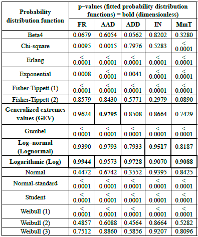
FR-frequency, AAD- annual average duration, ADD-annual daily duration, I- intensity, MmT-maximum maximorum temperature and (boxed and bold)-fitted probability distribution functions.

Source: ^{Llanes et al. (2021)}

Statistical analysis of the fitted probability distribution functions

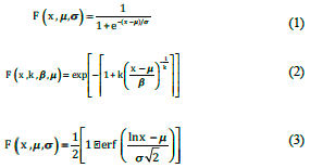
To obtain the fitted probability distribution functions of HE indicators and MmT, in this study the maximum likelihood estimation method was used. This mathematical method was applied due to its adaptability to the different HE indicators and its precision in the estimation of large samples (data series for the period 1982-2014; ^{Gómez, 2020}). The p-values of 16 probability distribution functions were calculated for the annual average values of each MeT indicator. This statistical method was used because is considered one of the most consistent, sufficient and asymptotically unbiased ways to identify the weather parameters of the fitted probability distribution functions (^{Strupczewski et al., 2001}). In addition to being more complex than the method of moments, it allows for greater rigor for all distributions (XLstat, 2022), and a greater reliability of fit for each indicator of HE and MmT. In this study, the fitted probability distribution functions used were logarithmic (Log), log-normal (Lognormal), and generalized extreme values (GEV) (^{Chow et al., 1994}; ^{Campos, 2016}). Log, lognormal and GEV functions are shown in Equations 1, 2 and 3, respectively. These calculations were carried out using XLstat version 2014.

Adjusted return periods

To obtain the cumulative distribution function F(x) of each fitted probability distribution function, the variable (x) and the following parameters were substituted into Equations 1, 2 and 3: the location (μ) and scale (σ) parameters in the log and lognormal functions; and the shape (k), scale (β) and location (μ) parameters into the GEV distribution. Equation 4 was used to calculate the adjusted return periods (ARPs, ^{Chow et al., 1994}; ^{Woong et al., 2003}). To calculate the frequency of occurrence (ARPs, Equation 4) of extreme events for each indicator of MeT, with Equations 1, 2 and 3, implicit in the function F(x), the values of the parameters μ, σ, k, and β , (obtained with the XLstat version 2014 software) were aggregated, respectively.

The modeling tools of this study (ST, fitted probability distribution functions and ARP), associated with the indicators of MeT; HE (Fr, AAD, ADD and IN) and MmT, serve to estimate the frequency of MeT occurrence. This methodology has also been applied by ^{Chow et al. (1994)}, ^{Ariza (2013)}, ^{Gomáriz (2015)} and ^{Campos (2016)}. To calculate the ARPs, XLstat version 2014, Surfer version 10.0 and corelDRAW version X7 were used.

3. Results and Discussion

3.1 Mann-Kendall test for STs

Figure 2 shows the weather stations with warming or cooling STs (ST positive or ST negative, respectively) of the indicators of MeT; FR, AAD, ADD, IN and MmT. The number of negative and positive STs for indicators of MeT were FR 6 negative and 3 positive; AAD 5 negative and 3 positive; ADD 6 negative and 3 positive; IN 5 negative and 4 positive; and MmT 6 negative and 3 positive. The weather stations that showed negative STs in the five MeT indicators were JAI, OTA and ROS, and the highest value of ADD was recorded at the ROS station with ST=-3.60. Only one station showed a highest positive ST in the five MeT indicators; namely, GUT with ST=3.90. These results are consistent with those of ^{Llanes et al. (2015)} in that although these authors calculated trends for the annual average maximum temperature, they also found a negative ST at the JAI station and a positive ST at the GUA station. These results provide essential information to characterize the evolution of regional warming-cooling, which should be attributed, according to ^{Alghamdi and Harrington (2019)}, not only to local and regional changes (elevation, latitude, and proximity to water bodies), but also to synoptic scale changes (atmospheric circulation) such as the climate indices Pacific decadal oscillation, Atlantic multidecadal oscillation, oceanic El Niño index and North Atlantic oscillation (Llanes, 2023).

Figure 2 Interpolation of Mann-Kendall test (STs = black line, dimensionless). 

Sen's slope test for STs

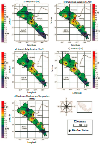
Figure 3 shows the magnitudes of the ST indicators. The highest magnitudes of negative ST were recorded at stations EPL (FR = -2.81 HE dec^-1, AAD = -9.38 day HE^-1 dec^-1 and MmT = -1.88 °C day^-1 dec^-1), ACA (ADD = -20.94 day dec^-1) and BAD (IN = -12.92 °C dec^-1). The highest positive magnitudes of ST were recorded at stations CUL (FR = 3.44 HE dec^-1), GUT (AAD = 6.15 day HE^-1 dec^-1 and IN = 13.62 °C dec^-1), IXP (ADD = 35.00 day dec^-1) and POT (MmT = 2.50 °C day^-1 dec^-1), as shown in Figure 3. If Li's criteria are considered, which are applied in the presence of extreme droughts, the positive trends of STs om FR, AAD, ADD, IN, and MmT suggest that extreme drought events may occur near stations CUL, GUT, IXP and POT. In this situation, the strength of these events could affect the yield of priority rainfed crops grown in the study area; beans, sorghum (Sagarpa, 2015) and corn (^{Llanes et al., 2022b}). This is verified with the results obtained by Llanes et al. (2022b), who established that in Sinaloa, the indices of meteorological drought that require evapotranspiration and maximum temperature as input data for their calculation (i.e., reconnaissance drought index and effective reconnaissance drought index) registered the highest significant correlations with rainfed maize yield; i.e., in Las Tortugas (station with the highest average maximum temperature for the period 1982-2013). This could put the socioeconomic and agrifood sustainability of Sinaloa and the whole country at risk (^{Robeson, 2004}; ^{Ruiz et al., 2005}; ^{Sheridan & Lee, 2018}), especially considering that this is one of the most important agricultural states in Mexico (^{Rincón, 2012}). In summer, Sinaloa has extremely high temperatures (up to 48 °C) and is often affected by diseases caused by high MeTs (^{Riojas et al., 2006}). It is important to note that the positive values of ST for MmT suggests that the people near stations CUL, GUT, IXP and POT could be at risk of sporadic events of heatstroke and, as a consequence, potential loss of human life (OPS, 2019).

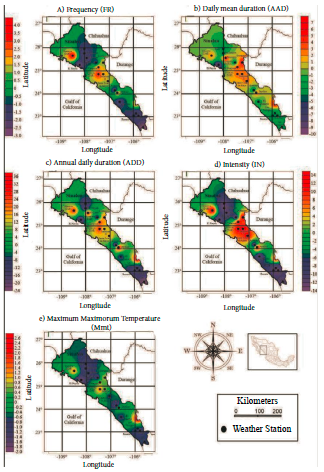
Figure 3 Interpolation of Sen's slope test (STs = black line). Measurement units: a (HE dec^-1), b (day HE^-1 dec^-1), c (day dec^-1), d (°C dec^-1) and e (°C day^-1 dec^-1). 

The results of the analysis of FR, AAD, ADD, IN and MmT presented in Table 3 show a prevailing cooling trend, due to the number of indicators of MeT with negative STs (28 stations) being greater in absolute value than those with positive values (15 stations).

Table 3 Location, scale, and shape parameters of the fitted probability distribution 

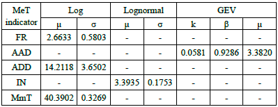
MeT-maximum extreme temperature, FR-frequency, AAD- annual average duration, ADD-annual daily duration, I-intensity, MmT-maximum maximorum temperature, Log-logarithmic, Lognormal-Log-normal, GEV-generalized extreme values, u-location, o-scale, k-shape and P-scale.

Source: ^{Llanes et al. (2021)}

These results are consistent with the historical evidence reported by ^{Llanes et al. (2015)}, where they found a higher number of weather stations with negative STs for the minimum temperature in the states adjacent to Sinaloa (Baja California Sur, Durango, Chihuahua, and Sonora). Of 38 weather stations studied, 20 showed negative STs and 18 positive STs. Llanes et al. (2015), found that in some stations near the state of Sinaloa there are negative trends for the minimum and average temperatures, but not for the maximum temperature, which presents a positive trend (i.e., in the stations Puerto San Carlos, El Rosario and Ojito de Camellones), which can be attributed to the high randomness between the spatial and temporal influence of the Pacific decadal oscillation, Atlantic multidecadal oscillation, oceanic El Niño index, North Atlantic index, and geopotential height at the level of 700 hPa (Llanes et al., 2018; Llanes et al., 2020; Llanes, 2023), and the magnitudes of the maximum, minimum and average temperatures, and the meteorological droughts of the northern states of Mexico (Llanes et al., 2018).

The difference between Figures 2 and 3 is that Figure 2 only identifies which indicators are statistically significant and Figure 3 shows the amount of significant trend.

Statistical analysis of the fitted probability distribution functions

Table 2 shows the p-values of the fitted probability distribution functions, where the maximum values correspond to the Log, GEV and Lognormal functions. The highest p-values of the MeT indicators were FR (Log, p=0.9944), AAD (GEV, p=0.9795), ADD (Log, p=0.9728), IN (Lognormal, p=0.9517 and MmT (Log, p=0.9088). The lowest p-values (p < 0.00001) corresponded to the fitted probability distribution functions Erlang, Fisher-Tippett (1), Gumbel, Normal-standard, Student and Weibull (1). If the log function were chosen for all the indicators (FR, AAD, ADD, IN and Mmt), then even the indicators AAD and IN (which do not present large p-values) can show good fit (p = 0.9573 and p = 0.9070 respectively).

These results are in agreement with ^{Aguilera (2007)} and with ^{Papacharalampous et al. (2018)}, who states that hydroclimatological data are rarely normally distributed; MeT indicators theoretically fit distributions that represent seasonal extreme values (^{Linsley et al., 1977}; ^{Pliego & Ruiz 2004}; ^{Campos 2014}; ^{Wang et al., 2016}; ^{Alghamdi & Harrington, 2019}).

Adjusted return periods

Table 3 shows the magnitudes of the shape, scale and location parameters of the fitted probability distribution functions used to calculate the adjusted return periods (ARPs). These parameters, based on the average values of MeT, are shown in Figure 4 for the ranges FR, 1.07 to 377.84 years; AAD, 1.03 to 24.88 years, ADD 1.06 to 816.94 years, IN, 1.02 to 16.59 years; and MmT, 1.03 to 118.15 years.

The P85 of MeTs as a function of the ARPs are FR (P85=3.65 HE year^-1; Figure 4a), AAD (P85= 5.09 day HE^-1 year^-1; Figure 4b),ADD (P85=19.34 day^-1 year^-1; Figure 4c), IN (P85=36.99 ^oC year^-1; Figure 4d), and MmT (P85=40.85 °C day^-1; Figure 4e).

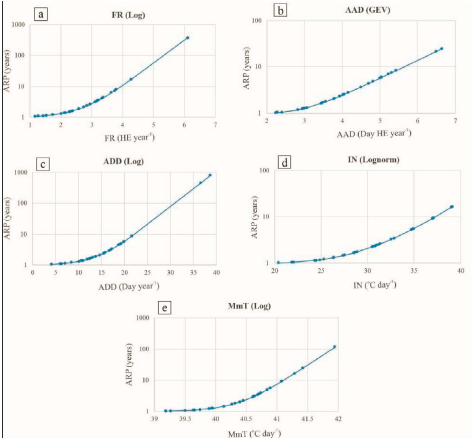
Figure 4 Adjusted return periods (ARPs) of the maximum extreme temperature (MeT) indicators: hot extremes (FR, frequency; AAD, annual average duration; ADD, annual daily duration; IN, intensity) and maximum maximorum temperature (MmT). Fitted probability distribution functions: logarithmic (Log), Lognormal (Log-normal) and generalized extreme values (GEV).  

According to Figure 4, the average occurrence frequency of extreme events (values with the highest probability of exceedance) per 100 years are FR = 1.16 HE dec^-1 (ARP = 1.07 years; prob. = 0.93 = 93 times ), AAD = 2.24 day HE^-1 dec^-1 (ARP = 1.03 years; prob = 0.97 = 97 times), ADD = 4.16 day dec^-1 (ARP = 1.06 years; prob = 0.94 = 94 times), IN = 20.42 °C dec^-1 (ARP = 1.02 years; prob = 0.98 = 98 times) and MmT = 39.18 °C day^-1 dec^-1 (ARP = 1.03 years; prob = 0.98 = 98 times).

The average frequency of occurrence of extreme events (values with less probability of exceedance) per 100 years are FR = 6.11 HE dec^-1 (ARP = 377.84 years; prob. = 0.01 = 1 time), AAD = 6.64 day HE^-1 dec^-1 (ARP = 24.88 years; prob = 0.04 = 4 times), ADD = 38.68 day dec^-1 (ARP = 816.94 years; prob = 0.01 = 1 time), IN = 39.09 °C dec^-1 (ARP = 16.59 years; prob. = 0.06 = 6 times) and MmT = 41.95 °C day^-1 dec^-1 (ARP = 118.15 years; prob. = 0.01 = 1 time).

These results are especially useful for carrying out adaptation measures in sectors such as the agrifood industry, which is the main economic activity in the state of Sinaloa (^{Fiscal et al., 2017}).

If these results are not considered in the decision making for seeding and harvesting dates, significant reductions in crop yields could occur in the region, resulting in significant negative effects on the economy of the region, which can generate high costs (^{Ruiz et al., 2013}; ^{Llanes et al., 2022b}). These unusual temperature fluctuations (indicators of MeT) that will increase by the year 2030 (World Bank et al., 2014), could trigger significant decreases in agricultural crop yields in Sinaloa (Llanes et al., 2022b), which will aggravate the food sustainability of Sinaloa and of Mexico.

Through the results of this study, the association among the indicators of MeT can be observed; HE (FR, AAD, ADD and IN) and MmT and the modeling tools (STs, fitted probability distribution functions and ARPs), which satisfy the requirements for calculating estimates of the frequency of occurrence of MeT indicators.

Source: ^{Llanes et al. (2021)}

4. Conclusions

Based on the ST results of these parameters, a greater number of negative values were observed than positive, which shows a trend toward cooling. The fitted probability distribution functions used to calculate the indicators of MeT were for FR, Log; for AAD, GEV; for ADD, Log; for IN, Lognormal; and for MmT, Log. This contribution provides a useful methodological tool to design adaptation strategies for climate change and natural disasters that may affect the agrifood sector. With the strategies that can be devised, non-reduction of the agricultural yield should be guaranteed for the most important crops in Sinaloa; maize, sorghum, wheat, and beans. These products are a mainstay in feeding Mexico and a great part of the harvest comes from the study area, which is still called "the breadbasket of Mexico." Limitations of this study are the small number of weather stations studied and the small number of probability distribution functions used for the fit. It is recommended that the MeT indicators be recalculated with data from a greater number of meteorological stations, as well as using a greater number of probability distribution functions to try to increase the p-values and obtain more accurate ARP. Some proposals for climate-smart agricultural strategies (adaptation/prevention) are drip irrigation, protected agriculture, and crop substitution, which can serve to minimize the effects of high temperatures in the agricultural activities of Sinaloa state.

References

Aguilera, N. M. A. (2007). Estimación de funciones de distribución de probabilidad, para caudales máximos, en la región del Maule. Memoria de la Universidad de Talca. [ Links ]
Alghamdi, A. S., & Harrington, J. J. (2019). Trends and spatial pattern recognition of warm season hot temperatures in Saudi Arabia. Theoretical and Applied Climatology, 138, 793-807. https://doi.org/10.1007/s00704-019-02860-6Links ]
Alves, M., Nadeau, D. F., Music, B., Anctil, F., & Fatichi, S. (2021). Can we replace observed forcing with weather generator in land surface modeling? Insights from long-term simulations at two contrasting boreal sites. Theoretical and Applied Climatology , 145, 215-244. https://doi.org/10.1007/s00704-021-03615-yLinks ]
Ariza, R. A. M. (2013). Métodos utilizados para el pronóstico de demanda de energía eléctrica en sistemas de distribución. [Tesis de Licenciatura, Universidad Tecnológica de Pereira], 145p. [ Links ]
Austin, C. P., & van Buuren, S. (2022). The effect of high prevalence of missing data on estimation of the coefficients of a logistic regression model when using multiple imputation. BMC Medical Research Methodology, 22, 196. https://doi.org/10.1186/s12874-022-01671-0Links ]
Blanco, M. E., Vaquera, H., Villaseñor, J. A., Valdez, L. J. R., & Rosengaus, M. (2014). Metodología para investigar tendencias espacio-temporales en eventos meteorológicos extremos: caso Durango, México. Tecnología y Ciencias del Agua, 5(6), 25-39. http://www.scielo.org.mx/pdf/tca/v5n6/v5n6a2.pdfLinks ]
Campos, A. D. F. (2014). Estimación probabilística de crecientes estacionales con base en registros mensuales de gasto máximo. Tecnología y Ciencias del Agua , 5(6), 177-18. http://www.scielo.org.mx/scielo.php?script=sci_abstract&pid=S2007-24222014000600013&lng=es&nrm=iso&tlng=esLinks ]
Campos, A. D. F. (2016). Ajuste de distribuciones GVE, LOG y PAG con momentos L de orden mayor. Ingeniería, Investigación y Tecnología, 17(1), 131-142. http://www.scielo.org.mx/scielo.php?pid=S1405-77432016000100131&script=sci_abstractLinks ]
Chapman, S. C., Watkins, N., & Stainforth, D. A. (2019). Warming trends in summer heatwaves. Geophysical Research Letters, 46, 1634-1640. https://doi.org/10.1029/2018GL081004Links ]
Chow, V. T., Maidment, R. D., & Mays, W. L. (1994). Hidrología aplicada. 584 pp. https://es.slideshare.net/LuigiQuispeYanapa/hidrologia-aplicada-ven-te-chow-116834237Links ]
CLImate COMputing (CLICOM) data base. Available online: Available online: http://clicom-mex.cicese.mx/mapa.html (accessed on 17 September 2021). [ Links ]
Cohen, J. L., Furtado, J. C., Barlow, M., Alexeev, V. A., & Cherry, J. E. (2012). Asymmetric seasonal temperature trends. Geophysical Research Letters , 39(4). https://doi.org/10.1029/2011GL050582Links ]
Demisse, M. U., Addisu, L. S., Bazezew, B. A., & Azhar, E. M. (2022). Climate Change Repercussions on Meteorological Drought Frequency and Intensity in South Wollo, Ethiopia. Earth Systems and Environment, 6, 645-655. https://doi.org/10.1007/s41748-022-00293-2Links ]
Deng, P., & Zhu, J. (2021). Forecast and uncertainty analysis of extreme precipitation in China from ensemble of multiple climate models. Theoretical and Applied Climatology , 145, 787-805. https://www.researchsquare.com/article/rs-209537/v1Links ]
Fiscal, C. B., Restrepo, B. L. F., & Rodríguez, E. H. (2017). Estructura productiva agrícola del estado de Sinaloa, México, y el tratado de libre comercio de América del Norte (TLCAN). Chilean Journal of Agricultural & Animal Sciences, ex Agro-Ciencia, 33(1), 14-23. https://scielo.conicyt.cl/scielo.php?pid=S0719-38902017000100102&script=sci_abstractLinks ]
Flores, C. L. M., Arzola, G. J. F., Ramírez, S. M., & Osorio, P. A. (2012). Repercusiones del cambio climático global en el estado de Sinaloa, México. Cuadernos de Geografía - Revista Colombiana de Geografía, 21(1), 115-129. https://www.redalyc.org/pdf/2818/281822849009.pdfLinks ]
Fontanelli, O., Mansilla, R., & Miramontes, P. (2019). Distribuciones de probabilidad en las ciencias de la complejidad: una perspectiva contemporánea. Interdisciplina, 8(22), 11-37. https://doi.org/10.22201/ceiich.24485705e.2020.22.76416Links ]
Franzke, C. L. E. (2015). Local trend disparities of European minimum and maximum temperature extremes. Geophysical Research Letters , 42, 6479-6484. https://doi.org/10.1002/2015GL065011Links ]
Garry, F. K., McDonagh, E. L., Blaker, A. T., Roberts, C. D., Desbruyères, D. G., Frajka, W. E., & King, B. A. (2019). Model-derived uncertainties in deep ocean temperature trends between 1990 and 2010. Journal of Geophysical Research: Oceans, 124, 1155-1169. https://agupubs.onlinelibrary.wiley.com/doi/full/10.1029/2018JC014225Links ]
Ghasemi, A. R. (2015). Changes and trends in maximum, minimum and mean temperature series in Iran. Atmospheric Science Letters, 16(3), 366-372. https://doi.org/10.1002/asl2.569Links ]
Gomáriz, G. C. (2015). Estudio de sostenibilidad energética para una piscina de altas prestaciones. [Bachelor's thesis, Universidad Politénica de Catalunya], 95 p. [ Links ]
Gómez, M. A. (2020). Modelo de máxima verosimilitud. Libre empresa, 17(2), 121-138. https://doi.org/10.18041/1657-2815/libreempresa.2020v17n2.8027Links ]
González, C. J. M., Pérez, R. P., & Ruelle, P. (2011). Estimación de índices normalizados de lluvia mediante la distribución gamma generalizada extendida. Tecnología y Ciencias del Agua , vol. II, núm. 4, Oct.-Dec., 65-76. [ Links ]
Gudko, V., Usatov, A., Ioshpa, A., Denisenko, Y., Shevtsova, V., & Azarin, K. (2021). Agro-climatic conditions of the Southern Federal District of Russia in the context of climate change. Theoretical and Applied Climatology . https://doi.org/10.1007/s00704-021-03677-yLinks ]
Gurung, B., Sarkar, K. P., Singh, K. N., & Lama, A. (2021). Modelling annual maximum temperature of India: a distributional approach. Theoretical and Applied Climatology , 145, 979-988. https://doi.org/10.1007/s00704-021-03674-1Links ]
Habibi, B., & Meddi, M. (2021). Meteorological drought hazard analysis of wheat production in the semi-arid basin of Cheliff-Zahrez Nord, Algeria. Arabian Journal of Geosciences, 14, 1045. https://doi.org/10.1007/s12517-021-07401-yLinks ]
Hochman, A., Marra, F., Messori, G., Pinto, J. G., Raveh, R. S., Yosef. Y., & Zittis, G. (2022). Extreme weather and societal impacts in the eastern Mediterranean. Earth System Dynamics, 13, 749-777. https://doi.org/10.5194/esd-13-749-2022 [ Links ]
Horton, R. M., Mankin, J. S., Lesk, C., Coffel, E., & Raymond, C. (2016). A review of recent advances in research on extreme heat events. Current Climate Change Reports, 2, 242-259. https://doi.org/10.1029/2018JC014225Links ]
Instituto Nacional de Estadística y Geografía (Inegi). (2016). Anuario Estadístico y Geográfico de Sinaloa. http://estadisticas.sinaloa.gob.mx/documentos/AnuarioEstad%C3%ADsticoSinaloa2016.pdfLinks ]
Jaiswal, R. K., Lohani, A. K., & Galkate, R. V. (2023). Rainfall and Agro Related Climate Extremes for Water Requirement in Paddy Grown Mahanadi Basin of India. Agricultural Research, 12(1), 20-31. https://doi.org/10.1007/s40003-022-00629-4Links ]
Kendall, M. G. (1975). Rank Correlation Measures. London: Charles Griffin. https://www.worldcat.org/title/rank-correlation-methods/oclc/3827024Links ]
Kienzle, W. S. (2018). Has it become warmer in Alberta? Mapping temperature changes for the period 1950-2010 across Alberta, Canada. The Canadian Geographer/Le Geographe Canadien, 62(2), 144-162. https://doi.org/10.1111/cag.12432Links ]
Kumar, U., Kumar, S. D., Chandra, P. S., Kumar, B. J., & Kant, L. (2023). Spatio-temporal trend and change detection of rainfall for Kosi River basin, Uttarakhand using long-term (115 years) gridded data. Arabian Journal of Geosciences , 16, 173. https://doi.org/10.1007/s12517-023-11244-0Links ]
Latif, S., & Mustafa, F. (2020). Copula-based multivariate flood probability construction: a review. Arabian Journal of Geosciences , 13, 132. https://doi.org/10.1007/s12517-020-5077-6Links ]
Li, X., You, Q., Ren, G., Wang, S., Zhang, Y., Yang, J., & Zheng, G. (2018). Concurrent droughts and hot extremes in northwest China from 1961 to 2017. International Journal of Climatology, 39(4), 1-11. https://doi.org/10.1002/joc.5944Links ]
Linsley, R., Kohler, M., & Paulus, J. (1977). Hidrología para ingenieros. 2 ed. México. Editorial McGraw-Hill Latinoamericana. [ Links ]
Little, R. J. A., & Rubin, D. B. (1987). Statistical Analysis with MissingData. Wiley, New York 1987, 14, 278. https://www.jstor.org/stable/1165119Links ]
Llanes, C. O. (2023). Predictive association between meteorological drought and climate indices in the state of Sinaloa, northwestern Mexico. Arabian Journal of Geosciences , 16, 79. https://doi.org/10.1007/s12517-022-11146-7Links ]
Llanes, C. O., Gutiérrez, R. O. G., Montiel, M. J., & Troyo, D. E. (2022a). Hot extremes and climatological drought indicators in the transitional semiarid-subtropical region of Sinaloa, northwest Mexico. Polish Journal of Environmental Studies, 31(5), 4567-4577. https://doi.org/10.15244/pjoes/149882Links ]
Llanes, C. O., Norzagaray, C. M., Gaxiola, A., Pérez, G. E., Montiel, M. J., & Troyo, D. E. (2022b). Sensitivity of four indices of meteorological drought for rainfed maize yield prediction in the state of Sinaloa, Mexico. Agriculture, 12, 525. https://doi.org/10.3390/agriculture12040525Links ]
Llanes, C. O., Norzagaray, C. M., González, G. G. E., López, R. J. S. (2021). Análisis de efectos de indicadores de temperatura máxima extrema en el estado de Sinaloa. Congreso Internacional Academia Journals, Hidalgo, 956-960. [ Links ]
Llanes, C. O., Norzagaray, C. M., Muñoz, S. N. P., Ruiz, G. R., Troyo, D. E., & Álvarez, R. P. (2015). Hydroclimatic Trends in Areas with High Agricultural Productivity in Northern Mexico. Polish Journal of Environmental Studies , 24(3), 1165-1180. https://doi.org/10.15244/pjoes/31221Links ]
Lustenberger, A., Knutti, R., & Fischer, E. M. (2014). Sensitivity of European extreme daily temperature return levels to projected changes in mean and variance. Journal of Geophysical Research: Atmospheres, 119(6), 3032-3044. https://doi.org/10.1002/2012JD019347Links ]
Mann, H. B. (1945). Nonparametric tests against trend. Econometrica, 13, 245-259. https://www.jstor.org/stable/1907187Links ]
Murage, P., Hajat, S., & Kovats, R. S. (2017). Effect of night-time temperatures on cause and age-specific mortality in London. Environmental epidemiology, 1(2), e005. https://doi.org/10.1097/EE9.0000000000000005Links ]
Organización Panamericana de la Salud (OPS). (2019). Ola de calor y medidas a tomar. Revisión preliminar. 50p. https://www3.paho.org/hq/index.php?option=com_docman&view=download&alias=48467-heat-wave-and-measures-to-take-preliminary-review-spanish&category_slug=detection-verification-risk-assessment-1226&Itemid=270&lang=es [ Links ]
Papacharalampous, G., Tyralis, H., & Koutsoyiannis, D. (2018). Predictability of monthly temperature and precipitation using automatic time series forecasting methods. Acta Geophysica, 66, 807-831. https://doi.org/10.1007/s11600-018-0120-7Links ]
Pliego, J. M. & Ruiz, & M. L. (2004). Estadística I: Probabilidad. 2a ed. Madrid: Thomson. [ Links ]
Puerta, G. A. (2002). Imputación basada en árboles de clasificación. Eustat. https://www.eustat.eus/documentos/datos/ct_04_c.pdfLinks ]
Rincón, A. J. G. (2012). Sinaloa: 100 años de historia educativa 1910-2010. Universidad Pedagógica Nacional. https://es.scribd.com/document/370636982/libro-de-rincon-pdfLinks ]
Riojas, R. H., Hurtado, D. M., Idrovo, V. J., & Vázquez, G. H. (2006). Estudio diagnóstico sobre los efectos del cambio climático en la salud humana de la población en Mexico. Instituto Nacional de Ecología, Instituto Nacional de Salud Pública. [ Links ]
Robeson, S. M. (2004). Trends in time-varying percentiles of daily minimum and maximum temperature over North America. Geophysical Research Letters , 31(4). https://doi.org/10.1029/2003GL019019Links ]
Rojas, E., Arce, B., Pena, A., Boshell, F., & Ayarza, M. (2010). Cuantificación e interpolación de tendencias locales de temperatura y precipitación en zonas alto andinas de Cundinamarca y Boyacá (Colombia). Ciencia y Tecnología Agropecuaria, 11(2),173-182. http://www.redalyc.org/articulo.oa?id=449945029009Links ]
Ruiz, C. J. A., Medina, G. G., Macías, J. C., Silva, M. M. S., & Diaz, P. G. (2005). Estadísticas climatológicas básicas del estado de Sinaloa (Período 1961-2003). Libro Técnico Núm. 2. INIFAP-CIRNO. Cd. Obregón, Sonora, México. https://docplayer.es/41213292-Estadisticas-climatologicas-basicas-del-estado-de-sinaloa-periodo.htmlLinks ]
Ruiz, C. J. A., Medina, G. G., González, A. I. J., Flores, L. H. E., Ramírez, O. G., Ortiz, T. C., Byerly, M. K. F., & Martínez, P. R. A. (2013). Requerimientos agroecológicos de cultivos. Libro técnico Secretaría de Agricultura, Ganadería, Desarrollo Rural, Pesca y Alimentación (Sagarpa), 3, 578. https://www.researchgate.net/profile/Jose-Ruiz-Corral/publication/343047223_REQUERIMIENTOS_AGROECOLOGICOS_DE_CULTIVOS_2da_Edicion/links/5f1310e04585151299a4c447/REQUERIMIENTOS-AGROECOLOGICOS-DE-CULTIVOS-2da-Edicion.pdfLinks ]
Rustom, J. A. (2012). Estadística descriptiva, probabilidad e inferencia. Una visión conceptual y aplicada. Universidad de Chile. http://repositorio.uchile.cl/handle/2250/120284Links ]
Salgado, C. A., & Largo, O. J. (2018). Imputación de datos faltantes de temperatura máxima media mensual mediante métodos geoestadísticos en estaciones climáticas del Valle del Cauca en el periodo 2013-2014. [Bachelor's thesis, Universidad del Valle]. [ Links ]
Secretaría de Agricultura, Ganadería, Desarrollo Rural, Pesca y Alimentación (Sagarpa). (2015). Agenda técnica agrícola de Sinaloa. Segunda Edición. https://issuu.com/senasica/docs/25_sinaloa_2015_sinLinks ]
Sen, P. K. (1968). Estimates of the regression coefficient based on Kendall's tau. Journal of the American Statistical Association. 63, 1379-1389. https://www.pacificclimate.org/~wernera/zyp/Sen%201968%20JASA.pdfLinks ]
Seneviratne, S. I., Nicholls, N., Easterling, D., Goodess, C. M., Kanae, S., Kossin, J., Luo, Y., Marengo, J., McInnes, K., Rahimi, M., Reichstein, M., Sorteberg, A., Vera, C., & Zhang, X. (2012). Changes in climate extremes and their impacts on the natural physical environment. In: Field, C. B., Barros, V., Stocker, T. F., Qin, D., Dokken, D. J., Ebi, K. L., Mastrandrea, M. D., Mach, K. J., Plattner, G. K., Allen, S. K., Tignor, M., & Midgley, P. M. (eds.) Managing the Risks of Extreme Events and Disasters to Advance Climate Change Adaptation A Special Report of Working Groups I and II of the Intergovernmental Panel on Climate Change (IPCC). Cambridge University Press, Cambridge, UK, and New York, NY, USA, 109-230. [ Links ]
Seneviratne, S. I., Nicholls, N., Easterling, D., Goodess, C. M., Kanae, S., Kossin, J., Luo, Y., Marengo, J., McInnes, K., Rahimi, M., Reichstein, M., Sorteberg, A., Vera, C., & Zhang, X. (2012). Changes in climate extremes and their impacts on the natural physical environment. In: C. Field et al. (Eds.). Managing the Risks of Extreme Events and Disasters to Advance Climate Change Adaptation, A Special Report of Working Groups I and II of the Intergovernmental Panel on Climate Change (IPCC). Cambridge Univ. Press, Cambridge, U.K., and New York. pp. 109-230. https://www.ipcc.ch/site/assets/uploads/2018/03/SREX-Chap3_FINAL-1.pdfLinks ]
Sheridan, S. C., & Lee, C. C. (2018). Temporal trends in absolute and relative extreme temperature events across North America. Journal of Geophysical Research: Atmospheres , 123(11), 889-898. https://doi.org/10.1029/2018JD029150Links ]
Strupczewski, W., Singh, V., & Feluch, W. (2001). Non-stationary approach to at-site flood frequency modelling. Maximum likelihood estimation. Journal of Hydrology, 248, 123-142. https://doi.org/10.1016/S0022-1694(01)00397-3Links ]
Wang, J., Han, Y., Stein, M. L., Kotamarthi, V. R., & Huang, W. (2016). Evaluation of dynamically downscaled extreme temperature using a spatially-aggregated generalized extreme value (GEV) model. Climate Dynamics, 47, 2833-2849. https://doi.org/10.1007/s00382-016-3000-3Links ]
Woong, T. K., Yoo, C., & Valdés, J. B. (2003). Nonparametric Approach for Estimating Effects of ENSO on Return Periods of Droughts. KSCE Journal of Civil Engineering, 7(5), 629-636. [ Links ]
World Bank, CIAT, & CATIE. (2014). Agricultura climáticamente inteligente en Sinaloa, México. Serie de perfiles nacionales de agricultura climáticamente inteligente para América Latina. Washington D.C.: Grupo del Banco Mundial, 12p. https://cgspace.cgiar.org/bitstream/handle/10568/52994/CSA-en-Sinaloa-Mexico.pdf?sequence=7&isAllowed=yLinks ]
XLstat. (2022). Users manual. 1657p. https://cdn.xlstat.com/helpcentersfdc/XLSTAT_Help.pdf [ Links ]
Yuan, W., Cai, W., Chen, Y., Liu, S., Dong, W., Zhang, H., Yu, G., Chen, Z, He, H., Guo, W., Liu, D., Liu, S., Xiang, W., Xie, Z., Zhao, Z., & Zhou, G. (2016). Severe summer heatwave and drought strongly reduced carbon uptake in Southern China. Scientific Reports, 6, 18813. https://doi.org/10.1038/srep18813Links ]
How to cite item: Llanes-Cárdenas, O., Cervantes-Arce, L., & González-González G.E. (2023). Calculation of indicators of maximum extreme temperature in Sinaloa state, northwestern Mexico. Earth Sciences Research Journal, 27 (1), 77-84 https://doi.org/10.15446/esrj.v27n1.99036
Received: October 14, 2021; Accepted: April 10, 2023
*Corresponding author: ollanesc@ipn.mx
Creative Commons License This is an open-access article distributed under the terms of the Creative Commons Attribution License