1. Introduction
Water is one of the necessary resources for the continuity of life on the Earth. Water resources are in danger of extinction due to reasons such as increasing population, industrialization, evaporation and decrease in precipitation. Water started to be traded on the stock market for the first time, such as gold and oil, with the CME(Chicago Commodity Exchange) group, the world's largest stock market operator in the USA, opening California's $1.1 billion futures contracts based on water assets on December 7, 2020 (Independent Türkçe, 2021). It should be noted that despite the value of water, it becomes mixed with the oceans after precipitation and thus is no longer usable as fresh water. Among these reasons, 60.6% of the precipitation falling on land returns to the atmosphere as evaporation (Rodell et al., 2015).
Determining the amount of evaporation is one of the important parameters in the planning of water resources (Aydin, 2009) Evaporation is a key process in the hydrological cycle that has a direct impact on the planning and operation of water (Penman 1948; Stewart 1984). Therefore, accurate estimation of evaporation is very important for water engineers and managers (Qasem et al., 2019). After the stock market transaction, estimation has become important for stockbrokers as well.
Evaporation estimation from the free water surface can be classified into two groups as direct and indirect methods (Keskin and Terzi, 2005). The pan measurement method is known as the direct method. The methods developed as an alternative to evaporation measurement by the pan method are empirical (traditional) relations known as the indirect methods depending on meteorological parameters. Some parameters affecting evaporation in these empirical relations are precipitation, air temperature, water temperature, solar radiation, sunshine duration, relative humidity, air pressure and wind speed. Evaporation prediction is an interesting field of study because it has been studied for many years and remains up-to-date (Thanh et al., 2020; Sun et al. 2021). Evaporation estimation with artificial neural networks (ANN) is a frequently used method (Tajar et al., 2018; Gümü§ et al., 2016; Doğan, 2020; Kiçi and Afçar, 2010; Õzdülkar et al., 2019; Õzel and Büyükyildiz, 2019).
Researchers aim to find the systems that best represent the actual amount of evaporation by using different methods in water basins. It is not easy to reach this goal with high accuracy due to the excess and variability of effective parameters in water basins.
In this study, firstly, evaporation models were developed by using ANN because of its success in explaining nonlinear relationships with air temperature, water temperature, sunshine duration, and solar radiation parameters. Then, the norm operator was used to improve the performance of the developed ANN models. Fort this, correlation analysis was performed between meteorological input parameters, and N-ANN models were developed with new input parameters created by applying the norm operator among the highly correlated parameters.
2. Methods
2.1. Study Region and Data
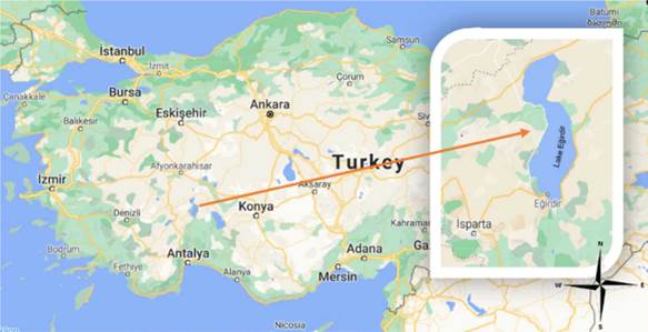
Lake Eğirdir is located within the borders of Isparta province in the Western Mediterranean part of Turkey (Figure 1). It is 917.7 m high, located at latitudes 35° 37' 41"-38° 16' 55" N and longitudes 30° 44' 39"-30° 57' 43" (Kesici and Kesici, 2006). With an area of 457 km2, it is the fourth largest lake in Turkey and the second largest in the Lake District (Şener et al.2013). The lake, which has steep rocks and a flat and shallow bottom, has a coastline of 150 km. The part located in the north of Kemer Strait in Lake Eğirdir is known as Hoyran, and the part in the south is known as Eğirdir.
The surface area of Lake Eğirdir varies depending on the water use. Some of the sinkholes, especially in the western parts of the lake, which has a karstic structure, have been closed. Numerous pumping stations have been established by General Directorate of State Hydraulic Works in the lake to be used for domestic usage, agriculture etc. Another of the most important features of Lake Eğirdir is its connection with the sea. There is the Kovada Canal of 22 km, which creates a natural connection between Lake Eğirdir and Lake Kovada. The water from Kovada Canal that flows into Kovada Lake is released from Kovada Valley into Aksu Stream and subsequently discharged into the Mediterranean through karstic pathways. Over the past two decades, the water from the lake has been diverted to Karacaõren I and II Dams located on the Çandir Plain. Eğirdir Lake meets the drinking water needs of Isparta province and surrounding settlements. It is also used as irrigation water in the plains of Isparta, Gõnen, Uluborlu, Senirkent, Yalvaç, Gelendost and Eğirdir. Although the lake has a closed basin, it is fed with abundant spring waters from its bottom and 1/3rd of the lake water is renewed every year. In June and October, the annual average evaporation amount in Lake Eğirdir is 500-530 hm3. The lake is especially fed by groundwater at the bottom. There are also many streams in the area. The most important of these are Pupa Stream, which comes from Yalvaç district and flows into the lake from Gelendost district, and goes down to the lake through Akçay, Uluborlu and Senirkent districts, Degirmen Stream descending from Hoyran plain and Aksu Stream, which is connected to the lake by a channel from Aksu Stream (Kesici and Kesici, 2006).
In the study, 490 days of air temperature, water temperature, sunshine duration, solar radiation and pan evaporation data of Lake Eğirdir for the years 2000-2001 were used. Meteorological parameters were obtained from the Automated Groweather Meteorology Station installed on the shore of Lake Eğirdir. Pan evaporation data were obtained from the General Directorate of State Hydraulic Works. Evaporation is estimated using the ANN method in region.
3. Artificial Neural Network
ANN consists of simple elements working in parallel. Network functionality is largely determined by the connections between elements. A neural network can be trained to perform a specific function by adjusting the values of the connections between elements. Usually, neural networks are set or trained so that a particular target output. The network aims to minimize the sum of the squared differences between the target and output values based on the comparison of the output and target. ANN uses many such input/target output pairs to train a network. Collective training of the network proceeds by making weight and bias changes based on all the input vectors. Adaptive training changes the weights and biases of a network as needed after the presentation of each input vector. Neural networks are trained to perform complex functions in a variety of application areas, including pattern recognition, classification, speech, vision, and control systems. Today, neural networks can be trained to solve problems that are difficult for traditional computers or humans (Demuth and Beale 1998). Feed forward ANN models contain a neuron system organized in layers. There may be one or more hidden layers between the input and output layers. Neurons in each layer are connected to neurons in the next layer with weight w that can be adjusted during training. A data model containing x values presented in input layer i propagates over the network to first hidden layer j. Each hidden neuron receives w ¡j x ¡ . weighted outputs from neurons in the previous layer. These are summed to produce a net value that is then converted to an output value upon application of an action function (Imrie et al., 2000). A neuron consists of multiple inputs and a single output. The sum of the inputs and their weights results in an aggregation operation (Equation 1).
Here, w ij . is the built-in weight, x ¡ . is the input value and NET j . is the input value of a node in the layer.
The output of a neuron is decided by an activation function. Step, sigmoid, threshold, linear etc. are some special functions used in ANN models. The commonly used sigmoid activation function f(x), is formulated by Equation 2.
Back propagation learning algorithm is one of the most important historical developments in neural networks as it allows modeling and processing of many quantitative phenomena in the science and engineering area. This learning algorithm is applied to multilayer feed-forward networks consisting of processing elements with continuous and differentiable activation functions. Such networks associated with the back propagation learning algorithm are also called back propagation networks. Given a training set of input-output pairs, the algorithm provides a procedure for changing the weights in a backpropagation network to correctly classify the given input patterns. The basis of this weight update algorithm is the gradient descent method used for simple sensors with differentiable neurons. For a given input-output pair, the back propagation algorithm performs two phases of the data stream. First, the input pattern propagates from the input layer to the output layer, and as a result of this forward flow, it produces an output pattern with minimal frame differences between the output and target data. Then, the error signals resulting from the difference between the output pattern and the actual output are propagated back from the output layer to the previous layers to update their weights (Lin and Lee 1996). Various ANN methods are available such as multilayer perceptron neural networks (Kişi and Afşar, 2010) and radial basis function neural networks (Doğan ,2020). In complex problems encountered, a solution is sought for a single problem with different ANN methods. The relationship of the obtained methods is examined (Kişi and Afşar , 2010).
4. Norm Operation
The norm operator was applied to the original input data to improve the performance of the ANN method. In the norm operator, the data consisting of two different parameters are expressed with a point on the two-dimensional plane and the distances of these points to the center (0,0) point are determined. Then, norm-ANN (N-ANN) model is developed with the new input data.
Norm operator: Let K denote the field (set) of real or complex numbers and let X(x,y) be a vector space (subset) over the field K expressed by Equation 3.
function and for every (x,y)∈X and for every α∈K
If Equations 4, 5 and 6 are satisfied, the f function is a norm on the vector space X (Yildiz, 2005).
Euclidean norm: R 2 (Euclidean space) is a special vector space. The norm of a vector 𝑋𝑌 in this space with a starting point (x 1 , x 2 ) and an ending point (y 1 , y 2 ) is defined by Equation 8 and II 𝑋𝑌 II (Stewart, 2009).
Position vector: The position vector of any point X in a two-dimensional space is the vector denoted by (OX) whose starting point is the origin (0,0) and the end point is X(x,y). If the norm of this vector is
is a function defined by Equation 10 (Stewart, 2009). In the study, each data with two parameters can be expressed with a point in two-dimensional space. Each point expressed by parametric data can be mapped exactly to a position vector in two-dimensional space. The norms of the position vectors obtained as a result of this match, represent the input set of the norm ANN model to be created using the norm operator. The form of Equations 9 and 10 in four-dimensional space,
are expressed by Equations 11 and 12.
The f transformations given by Equations 10 and 12 satisfy the norm operator requirements given by Equations 5, 6 and 7. The norm operation is non-linear because it involves force. For this reason, norm calculation after normalization process for all data will provide more efficient results. k in the data group, with the maximum value of the F max data group and the minimum value of F min . normalization process for data,
is defined by Equation 13. The norm operator is used in many applied areas (Koksal et al.,2014).
5. Results and discussion
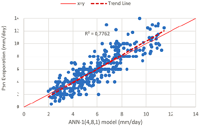
While developing the models, random 392 (80%) of the 490-day data were grouped as training set and the rest 98 (20%) as test set. In the first part of the study, evaporation models from the lake surface were developed by using the measured original air temperature (Ta), water temperature (Tw), sunshine duration (n) and solar radiation (Rc) parameters of Lake Eğirdir as inputs in the ANN. Statistical parameters of the best ANN models developed using tan-sigmoid transfer function (tansig) and feed-forward backpropagation algorithm are given in Table 1. According to Table 1, the determination coefficient (R2) was calculated using Equation 14 as 0.653 and the mean square error (MSE) value was calculated using Equation 15 as 1.360 for the test set of the best ANN-1 model.
Table 1 ANN model results
| Model | Network Structure* | Input Parameters | Training set | Test set | ||
|---|---|---|---|---|---|---|
| R2 | MSE | R2 | MSE | |||
| ANN -1 | (4,8,1) | Ta, Tw, n, Rc | 0.776 | 0.665 | 0.653 | 1.360 |
| ANN -2 | (4,10,1) | Ta, Tw, n, Rc | 0.762 | 0.653 | 0.624 | 1.853 |
| ANN -3 | (4,12,1) | Ta, Tw, n, Rc | 0.783 | 0.586 | 0.626 | 1.595 |
*Here the values in the brackets are the number of neurons as follow: Input layer, Hidden layer, Output layer.
where R i(real) and R i(model) are the real and estimated values, respectively.
The R𝑎𝑣𝑒𝑟𝑎𝑔𝑒 is the arithmetic mean of the real data.
*Here the values in the brackets are the number of neurons as follow: Input layer, Hidden layer, Output layer.
The scatter diagrams for the training and test sets of the ANN-1 model, which was chosen as the most suitable model, are given in Figures 2 and 3.
In the second part of the study, the norm operator was applied to the original input parameters to improve the performance of the ANN models. In order to decide with which parameters to develop the ANN models to be created using the norm operator, firstly, the R2 values between the input parameters were calculated and given in Table 2.
Table 2 The R2 relationship between parameters
| R 2 | Ta | Tw | n | Rc | Evap. |
|---|---|---|---|---|---|
| Ta | 1 | ||||
| Tw | 0.935 | 1 | |||
| n | 0.501 | 0.448 | 1 | ||
| Rc | 0.578 | 0.544 | 0.795 | 1 | |
| Evap. | 0.805 | 0.797 | 0.517 | 0.556 | 1 |
When Table 2 was examined, it was seen that the highest correlation was between Ta and Tw; n and Rc parameters. Based on the high relationship between Ta and Tw, the data of these two parameters were used in the norm operator after normalizing. In the same way, n and Rc parameters were also normalized and the norm operator was applied.
Based on the R2 values presented in Table 2, the Ta and Tw parameters have been selected which were found to have a strong correlation, along with the n and Rc parameters, for joint usage in our analysis. To calculate the Taw values, which is the norm value obtained using Ta and Tw, Equations (9) and (10) are utilized. Similarly, the other norm value called nRc has been calculated using n and Rc data. The resulting Taw and nRc values were incorporated into N-ANN models.
In addition to the binary combinations of the parameters, the four input parameters were converted into single parameters with the help of the norm operator. Here, the normalized air temperature (Ta), water temperature (Tw), sunshine duration (n) and solar radiation (Rc) values are called as TNR as domain elements of the f function defined by Equation (12). The parameterTNR=
 is obtained.
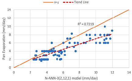
N-ANN models were created by using the new inputs (Taw and nRc) to which the norm operator was applied. For these N-ANN models, the tan-sigmoid transfer (tansig) function and feed-forward backpropagation algorithm are used. The results of the developed N-ANN models and the measured pan evaporation values were compared and the R2 and MSE values are given in Table 3. Among these models, it was seen that the most suitable model was the N-ANN-3 model with an R2 value of 0.722 and an MSE value of 2.314 for the test set.
Table 3 N-ANN model results
| Model | Network Structure* | Input Parameters | Training set | Test set | ||
|---|---|---|---|---|---|---|
| R2 | MSE | R2 | MSE | |||
| N- ANN -1 | (2,8,1) | Taw, nRc | 0.777 | 0.719 | 0.719 | 2.642 |
| N- ANN -2 | (2,10,1) | Taw, nRc | 0.762 | 0.741 | 0.646 | 2.642 |
| N- ANN -3 | (2,12,1) | Taw, nRc | 0.758 | 0.782 | 0.722 | 2.314 |
| N- ANN -4 | (2,13,1) | Taw, nRc | 0.771 | 0.723 | 0.697 | 3.313 |
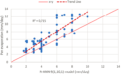
| N- ANN -5 | (1,10,1) | TNR | 0.733 | 0.945 | 0.715 | 2.874 |
*Here the values in the brackets are the number of neurons as follow: Input layer, Hidden layer, Output layer.
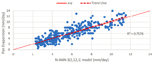
The scatter diagrams for the training and test sets of the N-ANN-3 model, which has two inputs among N-ANN models, are given in Figures 4 and 5.
Finally, the N-ANN-5 model was developed using four input parameters (Ta, Tw, n, Rc), the image set elements of the norm operator g function in four-dimensional space given in equation (12), and a single input parameter. The R2 value for the test set of this model was 0.733 and the MSE value was 2.87. It has been seen that the N-ANN-5 model developed with a single input gives similar results to the two-input models, and the scattering diagrams are given in Figures 6 and 7.
6. Conclusions
Determining the amount of evaporation from the water surface is very important in water planning and engineering calculations. Due to the variability of the multitude of effective parameters, it is laborious and difficult to determine the amount of evaporation by error-free and algebraic methods. For this reason, artificial intelligence methods, which are widely used in many fields recently, are preferred instead of direct measurement methods and empirical relations, which are difficult. ANN, one of the artificial intelligence methods, is one of the most frequently used methods in the field of hydrology. In this study, ANN models were created to estimate the amount of evaporation from Lake Eğirdir using the parameters of air temperature (Ta), water temperature (Tw), sunshine duration (n) and solar radiation (Rc). The original Ta, Tw, n and Rc parameters were first used to develop models with ANN. Then, by looking at the correlations of these input parameters, the related parameters were determined and after normalization, the norm operator was applied to the related parameters. After determining the related parameters Ta-Ts and n-Rc, each value is expressed as a vector and the lengths of these vectors are used as new input parameters to develop N-ANN models. In addition, a model was developed by transforming these four parameters into a single input parameter with the norm function and it was seen that it could be applied to higher dimensional data groups. When the developed models are compared, it is seen that the N-ANN models developed with the input parameters obtained after applying the norm operator gave more appropriate results.
In the study, the norm operator was used as a new method for data editing in evaporation estimation. When the literature is examined, it has been seen that ANN is frequently used for evaporation estimation. It is thought that converting multi-parameter data to real values with the norm operator and using it in ANN will contribute to the literature in data editing and pre-processing. Thus, it has been seen that modeling with the norm operator contributes to more accurate estimation.
For future studies, it is recommended to add the parameters precipitation and the relative humidity which are both important parameters for water budgeting as well. This will be investigated in the future studies.


