


 English (pdf)
 Article in xml format
 Article references
 Send this article by e-mail
 Cited by SciELO
  Cited by Google
  Similars in
SciELO
Similars in
SciELO  Similars in Google
 Permalink
I. INTRODUCTION
The study of mechanical impacts in physics has been of interest for decades, particularly collisions between small aggregates of dust grains (granular clusters). To model these clusters, one of the commonly used strategies is molecular dynamics (MD) simulations, which solve Newton’s equations of motion for an ensemble of particles interacting through a force field. This method allows incorporating complex properties of dust interactions. Typically, the grains themselves represent solid material that remains unchanged internally during the collision process, while the whole ensemble (the cluster) will undergo restructuring, aggregation, or fragmentation. This strategy has been used successfully to describe the collision of granular clusters containing up to several thousand grains [1].
MD granular simulations usually demand a high computational cost (in hardware and compute time) due to the number of objects simulated. For statistical analysis, it is always an advantage to decrease this time. ML supervised algorithms are good candidates for this purpose. The basic aim of these algorithms is to build predictive models, which attempt to discover and model the relationship between the predictor variable (independent variables) and the other variables. To build a predictive model, it is necessary to train the algorithm by giving instruction on what it needs to learn and how it is intended to learn it. Specifically, given a dataset, the learning algorithm attempts to optimize the model to find the combination of features that result in the target output. ML has been used successfully in combination with MD simulations in previous works such as: to accelerate ab initio MD simulations [2], to predict atomization energies in organic molecules [3], and to improve protein recognition [4], amongst others.
Machine learning is a branch of artificial intelligence interested in the development of computer algorithms for transforming data into intelligent action, and it has become the most popular and suitable tool for manipulating large data. The aim of machine learning is to uncover hidden patterns, unknown correlations and find useful information from data. Furthermore, it has extensively succeeded in performing predictive analysis [5], which is particularly of interest in this work.
For this work, the main purpose was to build such a model using ML algorithms to classify the grains of a collision, trying to find a “threshold time” for which the analyst knows with a certain accuracy what will be the outcome of the collision. With this threshold, the MD simulation can be stopped without simulating the entire collision process. It is expected that this cut time is shorter than the overall time of the simulation. The results showed that this method allows an improvement of at least more than 40 % of the total simulation time, which is encouraging.
This work is organized as follows. Section II presents a description of the type of granular simulations (subsection II-A) that are analyzed along with a description of the Machine Learning algorithm used (subsection II-B). The description of the software tools used can be seen in subsection II-C and the hardware used is in subsection II-D. The results and discussion are in section III. Finally, the main conclusions are in section IV.
II. MATERIAL AND METHODS
This section describes the type of granular simulations executed and the software that was used to perform them. Next, a description of the Machine Learning algorithms with their corresponding parameters is presented with the computational tools used.
A. Granular Mechanics Simulations
The collision of micro-metric dust grains is analyzed to find the speed limit that separates a process of agglomeration from the fragmentation. Understanding the mechanism of these processes in this scale is fundamental when trying to explain the formation of planetary rings, protoplanets, the distributions of powder grain sizes in different scenarios, etc. [6],[7].
Considering a model of granular matter where we incorporate cohesion forces [8], we perform simulations using Molecular Dynamics of collisions of porous grains composed of a Ni number of identical SiO2 particles of size 0.76 μm, where each grain has a variable fill factor between 0.15 and 0.35. We have studied the effect of the collision of two grains, a small one (the projectile) against a much larger one (the target), initially at rest. The projectile moves along the z-axis with a certain initial velocity between 0.1 and 1 m/s, and both the projectile and the target have the same filling factor (see figure 1). The filling factor is defined as the total grain volume of the number of grains Nδ in a sphere of radius δ around a certain grain i, divided by the sphere volume [9]. Once the projectile hits the target, the system is fragmented into two parts: one carried along by the projectile (blue grains in figure 1) and one that remains immobile (red grains in figure 1).
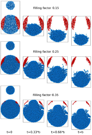
Fig. 1 Slice snapshots at different time steps (t=0 initial time step and tf final step) of granular simulations with three filling factors for the same initial velocity of 1m/s. Grains in different color indicate the two fragments at the end of the simulation.
The critical rate of fragmentation depends on the grain's filling factor and is the result of a “piston” effect that moves in a sustained manner some of the particles of the larger cluster. The usual models estimate that the minimum speed for grain fragmentation of these characteristics is of the order of 1-10 m/s [6],[10],[11]. In our work, we found fragmentation for speeds higher than 0.02 m/s, well below the previous estimates. We also found strong dependencies on fragment sizes with the filling factor, which has not been taken into account in current models. These results may involve modifications in the agglomeration/fragmentation models used.
The simulations were executed using LAMMPS (http://lammps.sandia.gov) in GPUs (Graphics Processing Unit). The granular pair style used was initially developed by Ringl et al. [8] to run in CPUs and later ported by Millán et al. [12] to run in NVIDIA GPUs with CUDA. As a reference, the simulations in GPU run ~3.6x times faster than in one CPU core and ~1.6x faster than 8 CPU cores (NVIDIA Titan Xp compared with an AMD EPYC 7281 CPU). More in-depth benchmarks can be seen in section III-B.
The granular simulations use input data generated with a model presented in [9] and a code developed by Millán and Planes (both authors of this work). The input data is composed of two spheres of grains: a projectile with a radius of ~14 μm and a target with a radius of ~31 μm. The samples have a filling factor of 15%, 25%, and 35%. The filling factor defines how much volume is occupied in both spheres (projectile and target). The number of grains in each simulation depends on the size of the spheres and the filling factor.
The simulations were configured to generate one dump file every 10000 steps. A dump file is a text file (with a format similar to csv or comma separated values with the configuration of the simulated system at a certain time step, including positions and velocities of each grain. For our simulations, each compressed (gzip) dump file sizes are between approx. 400 KB to 1000 KB (from 0.15 to 0.35 filling factor) and the number of dumps files generated varies between the different simulated configurations. Simulations with a faster velocity (1 m/s) ran fewer Total Steps than simulations with slower velocities (0.1 m/s), which needed more Total Steps to produce fragmentation. The total size of each compressed simulation varies from approx. 1 GB (0.15 fill factor for 1 m/s) to 8.5 GB (0.35 fill factor for 0.1 m/s) with a total of 42 GB of compressed data considering all 15 simulations tested in this work.
We performed the ML algorithms analysis on five different initial projectile velocities in small simulations, each with three filling factors (0.15, 0.25, and 0.35), giving a total of 15 simulations with different input conditions. These filling factors determined the total number of grains in each simulation (11200, 18785, and 26206 respectively). The same radius of the projectile was maintained in all three cases, and it represented around 9% of the total number of grains. Five projectile velocities were tested: 1.0, 0.75, 0.5, 0.25 and 0.1 m/s.
B. B. Machine Learning Algorithms
In this work, we have tested two supervised classification models: Support Vector Machine (SVM) and Random Forest(RF).
SVM is a class of powerful, highly flexible modeling techniques. It uses a surface that defines a boundary (called hyperplane) between various points of data leading to fairly homogeneous partitions of data according to the class labels (discrete attributes whose value is to be predicted based on the values of other attributes). SVM basic task is to find this separation among a set (sometimes infinite) of possibilities, choosing the Maximum Margin Hyperplane (MMH) that creates the greatest separation between classes. For no linearly separable data, a slack variable creates a soft margin, and a cost value C is applied to all points that violate these constraints, and rather than finding the maximum margin, the algorithm attempts to minimize the total cost. If the cost parameter is increased, it will be more difficult to achieve a 100 percent separation. On the other hand, a lower cost parameter will place emphasis on a wider overall margin. A balance between these two must be created in order to create a model that generalizes well to future data [13].
Random Forest is an ensemble-based method that focuses only on ensembles of decision trees (a recursive partitioning method that chooses the best candidate feature each time until a stopping criterion is reached). After the ensemble of trees is generated, the model uses a vote to combine the predictions. It is possible to define the number of decision trees in the forest and also how many features are randomly selected at each split. Random forests can handle extremely large datasets, but at the same time, its error rates for most learning tasks are on par with nearly any other method [13].
C. C. Computational Tools
Several computational tools were used in this work. To perform the granular simulations, the LAMMPS software was used, running primarily in GPUs. The generated output for each simulation is in a compressed gzip format to save disk space and transfer time between computers. The Classification Analysis was performed using the R language with several packages: dplyr for data manipulation, ggplot2 for plot generation, caret for machine learning algorithms, purrr to use the map() function and tictoc to easily measure compute time of sections of R code. The source code used to perform the analysis is available in the following url: https://sites.google.com/site/simafweb/.
The next subsection describes the hardware and software used to perform the granular simulations and the ML analysis.
D. Computational Tools
The MD simulations were executed using two different GPUs. The ML analysis was executed using one Workstation and the Toko cluster at FCEN-UNCuyo using only CPU cores. The following list details the hardware and software specifications:
Workstation FX-8350 with: AMD FX-8350 with 8 cores running at 4 GHz with 32 GB of DDR3 RAM memory. With one NVIDIA GeForce GTX Titan X (Maxwell GM200 architecture) with 12 GB of memory. Slackware Linux 14.2 64 bit operating system with kernel 4.4.14, OpenMPI 1.8.4, GCC 5.3.0, R language version 3.5.1, and Cuda 6.5 with NVIDIA driver 375.66.
Workstation FX-8350 with: same specifications than previous workstation but with a NVIDIA GeForce GTX Titan Xp (Pascal GP102 architecture) with 12 GB of memory.
Cluster Toko at the Universidad Nacional de Cuyo:
One node with four AMD Opteron 6376 CPU, with 16 CPU cores at 2.3GHz (each, 64 cores total), 128 GB of RAM, and Gigabit Ethernet.
One node with two AMD EPYC 7281 CPU, with 16 CPU cores at 2.1GHz (each, 32 cores total), 128 GB of RAM and Gigabit Ethernet.
Both nodes with Slackware Linux 14.1 64 bit with kernel 4.4.14, OpenMPI 1.8.8, GCC 4.8.2 and Cuda 6.5 with NVIDIA driver 396.26.
III. RESULTS AND DISCUSSION
In this section, the details of the performed simulations is described along with the ML analysis. Also, a small comparison of computational performance is shown for the hardware previously described.
A. A. Classification Analysis
Each simulation has a large number of output files (dump files or snapshots of the state of the simulations); we chose to apply the SVM and RF prediction algorithms to only 50 evenly spaced time steps of those output files. These algorithms were trained with the velocity in z as the predictor variable. The accuracy (number of correct classifications over the total number of grains) of each prediction is shown in detail in figure 2. As can be seen from the figure, as the initial velocity of the projectile increases, each test takes more steps to reach an accuracy of 90%. Also, for each speed, the 0.35 fill factor takes longer to reach this accuracy.
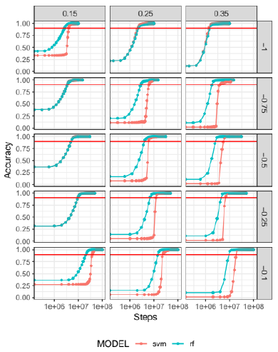
Fig 2 ML accuracy for 15 granular simulations with SVM (pink) and RF (blue) algorithms. Three filling factors are shown (0.15, 0.25 and 0.35) with five velocities (from -1 to -0.1 m/s). The dots represent 50 evenly spaced predictions for different time steps, to facilitate interpretation, the x-axis was rescaled with log function.
In general, the superiority of RF performance over SVM is evident. For lower speeds and higher fill factors, the SVM performance declines. We note in some cases, that the algorithms start with an accuracy higher than 0%. This is due to the predictor variable; the grains that belong to the projectile (in movement) and the grains belonging to the target which remains immobile throughout the collision are classified correctly at the initial step. For 0.35 fill factor, the amount of target grains that remain in the immobile fragment is very small, so the initial accuracy is quite poor.
Results of simulation time improvements are presented for two representative speeds and two fill factors in table 1. We define the gain percentage as the ratio of the time taken by the algorithms in reaching a prediction accuracy of 90% and the total computation time of the simulation. We have chosen this 90% accuracy value as a reference point from which predictions start to be reliable. Analysts will determine the best accuracy value suitable for their purposes, particularly if it is desired to analyze fragment sizes. For example, to obtain 99% accuracy in the case of 0.1 m/s initial velocity and a fill factor of 0.35, the gaining percentage is 79.7% using RF (90.6% with 90% accuracy) and 65.5% using SVM (80.4% with 90% accuracy).
TABLA I WALLCLOCK TIME (COMPUTATION TIME) FOR FOUR SELECTED GRANULAR SIMULATIONS COMPARED WITH THE TIME IT TOOK EACH ML ALGORITHM TO ACHIEVE A PREDICTION WITH A 90% OF ACCURACY. THE GAIN PERCENTAGE COLUMN SHOWS THE REDUCTION IN COMPUTE TIME THAT CAN BE ACHIEVE BY USING THE ML PREDICTIONS.
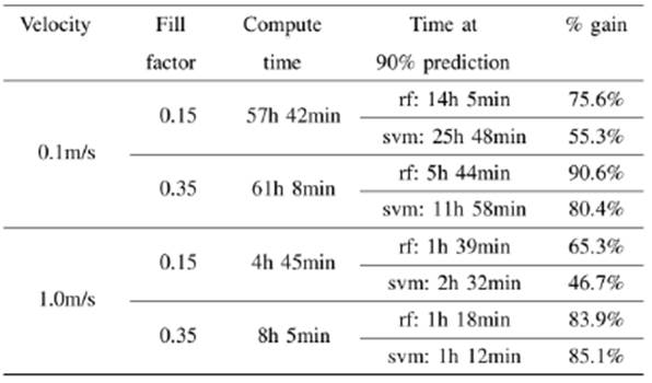
As can be seen from the table, in both velocities, the algorithms take longer to reach the 90% accuracy value for a 0.15 fill factor. We are currently working in the physics of this behavior in a work which is soon to be published.
As it was said previously, in general, RF has a better performance than SVM with a gap of 10% or more between gainings. The time it takes to train each algorithm is less than 1 minute, and the average time it takes to get the predictions of a file is less than 1 second, so they can be neglected.
B. B. Computational Benchmarks
Granular simulations were executed in two NVIDIA GPUs, the Titan X and Titan Xp; see subsection II-D for more information on hardware and software infrastructure. In this section, a comparison between CPU and GPU performance is shown. Figure 3 shows the performance of one granular simulation executed in two CPU nodes from Toko cluster from 1 to 32 CPU cores. For this size of simulation (11200 grains), the best performance is obtained with 16 CPU cores in both CPUs (AMD Epyc and Opteron). The Epyc processor is between ~1.5 and 2.1x times faster than the Opteron processor.
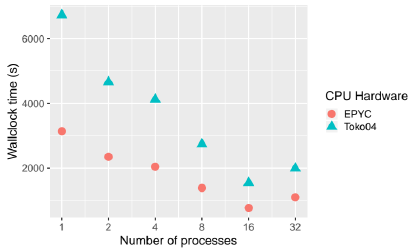
Fig. 3 Results for granular simulation with 11200 grains, velocity 5.0m/s and filling factor of 0.15, executed in two CPU cluster nodes from 1 to 32 cores. Time in seconds, lower is better.
For the same simulation shown in figure 3, the NVIDIA Titan Xp GPU has performance up to ~3.6x times faster than in one EPYC 7281 CPU core and ~1.6x faster than 8 EPYC 7281 CPU cores. The 16 EPYC CPU cores are ~1.1x faster than the Titan Xp GPU. The size of the simulations is not ideal for benchmarking, bigger simulations can produce a better performance speedup using GPUs. See [14] and [15] for more benchmarks.
IV. CONCLUSIONS AND FUTURE WORK
The computing time and HPC infrastructure needed to execute numerical simulations like the granular simulations presented in this work are a limiting factor for many researchers. Different tactics are required to reduce computational time or to improve the use of the available hardware infrastructure. Supervised ML algorithms used in this work were found suitable to build a predictive model to decrease simulation time. The overall results were encouraging: for the longest simulations, a potential 90% time reduction was achieved. The fill factor of the grains plays an important role in the algorithm’s prediction; for larger filling factors, the algorithms take more time to reach the desired accuracy.
As future work, we intend to try other suitable supervised algorithms and compare their performance with the ones used so far. We also plan to explore unsupervised algorithms such as DBSCAN [16], to improve the performance of SVM and RF. We also want to explore the dependence of the supervised algorithms with the different predictor variables (positions, velocities, angular velocities). An important subject that has to be addressed in future research is Transfer Learning, to be able to train the ML models with small simulations like the ones used in this work and make predictions about larger simulations.
We are also planning to use Hadoop with Mahout (https://mahout.apache.org/) to test SVM and RF (along with other algorithms) with granular simulations including 1e5 to 1e6 grains.

